J. Cent. South Univ. Technol. (2010) 17: 1310-1319

DOI: 10.1007/s11771-010-0636-8

Multi-label dimensionality reduction based on semi-supervised discriminant analysis

LI Hong(李宏), LI Ping(李平), GUO Yue-jian(郭跃健), WU Min(吴敏)

School of Information Science and Engineering, Central South University, Changsha 410083, China

? Central South University Press and Springer-Verlag Berlin Heidelberg 2010

Abstract: Multi-label data with high dimensionality often occurs, which will produce large time and energy overheads when directly used in classification tasks. To solve this problem, a novel algorithm called multi-label dimensionality reduction via semi-supervised discriminant analysis (MSDA) was proposed. It was expected to derive an objective discriminant function as smooth as possible on the data manifold by multi-label learning and semi-supervised learning. By virtue of the latent imformation, which was provided by the graph weighted matrix of sample attributes and the similarity correlation matrix of partial sample labels, MSDA readily made the separability between different classes achieve maximization and estimated the intrinsic geometric structure in the lower manifold space by employing unlabeled data. Extensive experimental results on several real multi-label datasets show that after dimensionality reduction using MSDA, the average classification accuracy is about 9.71% higher than that of other algorithms, and several evaluation metrices like Hamming-loss are also superior to those of other dimensionality reduction methods.

Key words: manifold learning; semi-supervised learning (SSL); linear discriminant analysis (LDA); multi-label classification; dimensionality reduction

1 Introduction

Traditional machine learning mainly resolves single-label learning problem, namely one sample only belongs to one class among the predefined classes. However, in real life one sample associated with multiple class labels always emerges, which is called as multi-label learning. It has been extensively applied in various areas, such as text classification, gene function analysis, image segmentation and video detection [1-2]. When it comes to high dimensional multi-label datasets, “curses of dimensionality” phenomenon happens. If no efficient feature extraction is done on the data, namely without dimensionality reduction, many original machine-learning methods would perform very poorly, especially large time and energy overheads might be required. On the contrary, it has been shown that performing dimensionality reduction, as a preprocessing step, would greatly improve the learning algorithms, e.g. extracting optimal representative features or transforming the original data into low-dimensional space via some algorithms [3-4].

Two well-known classical methods dealing with high-dimensional data are unsupervised primary component analysis (PCA) and supervised linear discriminant analysis (LDA). PCA performs dimensionality reduction by projecting the original n-dimensional data into the d (< In recent years, semi-supervised learning has attracted much attention in the field of machine learning. Usually, people can only obtain a very small number of labeled data samples while a large number of samples are unlabeled. In particular, it is a trivial and difficult task to label high-dimensional data [5]. As far as it concerns, many researchers have introduced the semi-supervised idea for dimensionality reduction, namely performing this task using both labeled and unlabeled data. ZHANG et al [6] used very few labeled samples to perform semi- supervised classification based on the canonical correlation analysis (CCA). CAI et al [4] presented a semi-supervised discriminant analysis method to deal with single labeled problem. SONG et al [7] put forward a unified framework for semi-supervised dimensionality reduction, under which PCA, LDA, MMC (maximum margin criterion), LPP and their corresponding kernel versions were all covered. CHENG et al [8] developed a semi-supervised dimensionality reduction method to balance the relevant feedback information in the image feature space. The above methods all aim at single-label problem, but luckily those methods have provided some useful minds for multi-label dimensionality reduction, which would be clearly shown in the following parts. Until now, there are only a few multi-label dimensionality reduction methods. YU et al [9] proposed a multi-label latent semantic index (MLSI) to preserve input information and capture correlations among multiple outputs. ZHANG and ZHOU [10] employed maximizing feature attributes and class label independence to perform multi-label dimensionality reduction (MDDM). PARK and LEE [11] exploited the generalized LDA to handle the multi-label problem and especially used the least squares regression to deal with high-dimensional multi-label text data. MLSI did not perform well due to its application constraints, and MDDM used all the label information that is often unavailable in real situations. Thus, a novel method called multi-label dimensionality reduction via semi-supervised discriminant analysis (MSDA) is presented, which only uses partial label information. The graph weighted matrix of sample attributes and the similarity correlation matrix of partial sample labels are employed to preserve global and local intrinsic geometry structure of the original data. MSDA combines semi-supervised learning and multi-label dimensionality reduction for the first time, which could be regarded as a developmental reference for the researches and applications of the high-dimensional data dimensionality reduction in future.

2 Multi-label classification

At present, there are two popular methods to deal with multi-label data. One is to decompose the multi-label classification task into a series of single-label problems, the other is to extend existing single-label methods to make it perform multi-label classification. BOUTELL et al [12] built the corresponding classifiers for every label to deal with multi-label scene classification, and those individual classifiers decided the output label sets of unlabeled data. This method did not consider the label correlations, and instead it assumed that all class labels were independent, which was always not true in reality. Later some methods exploiting the relationship among labels came into being. GODBOLE and SARAWAGI [13] aimed at balancing the label correlations by increasing background fusion based on individual classifiers. LIU et al [14] conducted semi- supervised multi-label learning by constrained non-negative matrix factorization. KANG et al [15] put forward a correlated label propagation (CLP) algorithm in order to acquire interaction among labels, and meanwhile CLP assisted to propagate label correlation information from training samples to testing samples. Recently, QI et al [16] employed the unified correlated multi-label support vector machine (CML-SVM) to perform classification, and built the model for label correlations in the new feature subspace. Essentially, the single-label problem is a special case of the multi-label problem. Thus, the multi-label problem is often converted to binary issue that is composed of both positive samples and negative samples. Every binary value corresponds to one label, and the generalized support vector machine and k nearest neighbor (kNN) classifiers are always used to accomplish multi-label classification tasks.

The mathematical definitions of multi-label classification are as follows. X={x₁, x₂, …, x_m} denotes a set of m-dimensional multi-label data samples, where each data sample is represented as a k-dimensional vector, namely x_i=[x_i1, x_i2, …, x_ik]^T, i=1, 2, …, m. It is also assumed that data samples have one or more class labels assigned among the predefined r classes. Let Y= {y₁, y₂, …, y_m} denotes the set of class labels for X. Each y_i=[y_i1, y_i2, …, y_ir] is a vector denoting class labels associated with x_i such that y_ij =1 if x_i belongs to class j, and y_ij=0 if x_i dose not belong to class j, where j=1, 2, …, r.

3 Linear discriminant analysis

Linear discriminant analysis attempts to find the optimal projection direction to a low-dimensional space, which would make those different classes as far away as possible while the same classes as close as possible. LDA utilizes the between-class scatter and the within-class scatter as a means to measure class separability. It is an ideal clustering structure for correct classification when the distance between classes is maximal and the distance within classes is minimal. The following will first review LDA for the single-label problem. The data set can be represented as X=  whereare the data samples belonging to class i and the total number of data is

The between-class scatter matrix S_b, the within-class scatter matrix S_w, and the total scatter matrix S_t are respectively defined as:

                     (1a)

                 (1b)

                   (1c)

where  denotes the class centroid of the ith class labels; and  denotes the global cen-

troid; S_b reflects the diversity among different samples; S_w reflects the subtle difference among samples with the identity labels; and S_t denotes the global difference among total ones. Generally, the between-class scatter and the within-class scatter could be measured by trace of a matrix. One of the optimization criteria is to find a linear transformation, which maximizes the ratio of the between-class scatter to the within-class scatter. That is:

            (2)

where for i=b or w, G^TS_iG is the scatter matrix. The total scatter matrix of all samples is the sum of the between- class scatter and the within-class scatter, which is denoted by S_t=S_b+S_w. So, actually resolving the optimal linear transformation is to obtain matrix G, which satisfies the objective function F_LDA(G) denoted as:

                    (3)

The issue becomes a non-zero eigen-problem if  J(S_b, S_w) is maximized. In other words, it aims at obtaining a group of eigenvectors g, which is composed of the columns of G. It is well known that LDA is a supervised method. When sufficient label information is available, it performs better than PCA. Nevertheless, when there is only a few label information, the estimated covariance matrices of sample class labels might be inaccuracy, which would possibly result in weak generalization ability on testing datasets. To solve this problem, labeled and unlabeled data samples could be considered together to help to find better projections in the low-dimensional subspace.

4 MSDA

Performing dimensionality reduction expects that the transformed data dimension in the low-dimensional subspace will be closer to the intrinsic dimension of the original data. The intrinsic dimension stands for the least dimension required to represent the high-dimensional data in the low dimensional manifold subspace [17]. As for the high-dimensional data, the ultimate goal for dimensionality reduction is that the linearly transformed data in the low-dimensional subspace can be very close to the intrinsic dimensions, preserving the global and local geometry structure. In practical applications, the labeled data are often very few. Therefore, it is the very research point that mining the latent correlated information hidden in a mass of unlabeled samples and preserving the intrinsic dimension as approximately as possible. A novel method for dimensionality reduction called MSDA was proposed to employ semi-supervised discriminant analysis on multi-label data. From perspective of graph in LDA, the multi-label problem can be regarded as an extension of single-label problem. The class label combination corresponding to one sample is treated as a new label, so referred notation r in the following parts represents the number of new label combinations. Every data sample could constitute vertices of the graph, and the relationship among data points is denoted by the edge weight. Thus, Graph can express the whole graph. While constructing the objective function of MSDA, both of the graph weighted matrix of attributes and the similarity correlation matrix of labels are considered.

4.1 Objective function

LDA aims at finding the projection vectors when the ratio of the between-class scatter to the total scatter achieves maximum. With regard to Eq.(1a), let c be zero, then:

                          (4)

where n denotes the number of labeled data samples; W ⁱ denotes a n_i×n_i matrix, where every element equals 1/n_i, and  denotes the data matrix of the ith class [6]. Let the data matrix X=[X¹, …, X^r], and a n×n diagonal matrix W_n×n is defined as

                   (5)

Then, Eq.(4) is equal to the following formula:

               (6)

Thus, Eq.(3) can be rewritten as:

                       (7)

When there are no sufficient training samples, namely samples are not typical, the over fitting phenomenon might happen. In order to prevent this case, the popular way is to impose a regularized function or factors. When introducing discriminant idea to the high-dimensional multi-label data, the label combinations are treated as a whole. Thus, if the helpful correlations among labels are not taken into account, this will certainly have influences on the performances of dimensionality reduction. MSDA exploits the similarity correlation matrix of labeled samples to eliminate over fitting, which will better preserve the intrinsic dimensional structure of the data. Thus, the objective function of MSDA is defined as:

          (8)

where H₁(G) and H₂(G) adjust the learning complexity of discriminant functions; and coefficients α and β control the balance between the model complexity and the empirical loss. MSDA employs the popular Tikhonov regularizer as control factors [6], denoted by H(G)= ||G||².

Useful prior knowledge on some particular applications can be incorporated into the objective function flexibly, with the help of the regularizer term H(G). As for the collected real high-dimensional dataset, only a few samples have labels. The goal of the regularizer is to make low-dimensional data preserve the primitive manifold structure. MSDA uses both labeled and unlabeled data for dimensionality reduction, in other words, it has introduced semi-supervised learning. Moreover, the key premise of semi-supervised learning is the prior assumption consistency of data points. For classification, nearby data have the same labels; for dimensionality reduction, neighboring data would have similar embeddings in the low-dimensional representations.

The mathematical definitions of MSDA are as follows. Given a k-dimensional multi-label dataset that is comprised of m data samples, in which n samples have labels. The total dataset is denoted by X=X_L+X_U and the label matrix is expressed by Y=[y₁, y₂, …, y_m], while the attribute matrix of labeled samples is denoted by X_L=[x₁, x₂, …, x_n} and unlabeled ones by X_U={x_n+1, x_n+2, …, x_m}. The main contribution of MSDA is that similarity correlation information provided by the label matrix is sophisticatedly used to perform dimensionality reduction, and the similarity correlation matrix is defined as: K_ij=||Y_il-Y_jl||² (i, j=1, …, n; l= 1, …, r). Matrix K_ij reflects the strong correlations among sample labels, which plays an important role in preserving geometry structure of the embedded manifold from high-dimension to low-dimension subspace. According to the theory of spectral dimensionality reduction, which plays a key role in spectral clustering and various kinds of graph based semi-supervised learning algorithms, there exists inevitable and essential relationship between sample labels and attributes. Motivated by this, a natural regularizer H₁(G) can be derived as follows:

                (9)

The algorithm uses a p-nearest neighbor graph Q= (V, E) to model the relationship among nearby data points, where V denotes the set constituted by the graph vertices, actually they are data samples, and E denotes the set constituted by the graph edges. If and only if two data points are neighbors, an edge may connect them. Moreover, different weights corresponding to different neighborhoods would be assigned to the edges between data points. Similarly, it is easy to represent the whole multi-label dataset as a weighted adjacency graph, which is defined as:

    (10)

where t denotes the Euclidean distance square centroid of all data points; N_p(x_i) denotes the set of p-nearest neighbors of x_i; and N_p(x_j) denotes the set of p-nearest neighbors of x_j. Generally, the mapping function should be as smooth as possible on the adjacency graph. In special, when two samples are linked by an edge, they are very likely to have the same class label set. Similar to H₁(G), another regularizer H₂(G) can be defined as:

               (11)

Then, two regularizers H₁(G) and H₂(G) are described as follows:

 (12a)

(12b)

where K and S are symmetric matrices; while D₁ and D₂ are diagonal matrices, whose entries are column sums of

K and S, respectively, denoted by D_1ii= D_2ii= According to the Laplacian theory, it can derive

L₁=D₁-K and L₂=D₂-S from the referred symmetric and diagonal matrices. With the assistance of the above two dependent regularizers, it can readily lead to the objective function MSDA as follows:

   (13)

4.2 Solutions to eigen-problem

Based on the linear algebra knowledge, Eq.(13) can be treated as solving an eigen-problem actually. Through computing the maximum eigenvalue of the generalized eigenvalue problem, the objective function could reach maximization. Meanwhile, it can acquire a series of projection vectors G_i, which just constitute the dimension transformation matrix G′. This generalized eigenvalue problem can then be transformed to solve the following equation:

  (14)

With regard to the whole samples, MSDA employs both labeled and unlabeled samples. Therefore, in order to maintain the consistency of the data matrix rank, both of matrices L₁ and W_n×n have to perform zero extensions. Thus, ranks of the new extended matrix and the corresponding total matrix are identical. Now, define L′ as the extended matrix of L₁ and W′ as the extended matrix of W_n×n. Then, we get:

, 

Let L=L₂, and the formula about the whole sample data can be yielded. Now, Eq.(14) can be rewritten as:

          (15)

And for Eq.(7), S_b=XW′X ^T and S_t=XI′X ^T can be obtained, and Eq.(15) is expressed in another form as follows:

   (16)

where

.

Thus, Eq.(16) can be simplified as:

          (17)

and it is equivalent to the equation:

.

Assume that A=(X(I′+βL)X^T)^-1X(W′+αL′)X^T, then the above equation turns to AG=λG. Herein, the problem of solving objective function is transformed to resolve the eigenvalues and eigenvectors of this formula AG=λG. From the clear analysis in the previous part, it is true that Rank(W′)=Rank(W)=r. So, with regard to a group of eigenvalues λ₁,…, λ_r, the corresponding eigenvectors G₁, …, G_r can be easily obtained. In theory, every dataset can be represented as the intrinsic dimensional structure in the low-dimensional subspace. At present, many intrinsic dimension estimation methods have been proposed, such as MLE (maximum likelihood estimator), GMST (geodesic minimum spanning tree), and Eigenvalue [2, 16-17]. Let the intrinsic dimension of X be d_im, then rank the output eigenvalues downwards, and choose those eigenvecters corresponding to the largest d_im eigenvalues to constitute the transformed matrix G′, denoted as G′=[G₁, …,  with the size of k×d_im. As a result, the original high-dimensional data can be transformed to low-dimensional data through this equation: Z=XG′, where the size of X is m×k while Z is m×d_im. In other words, the k-dimensional data have been transformed to d_im-dimensional data.

Generally, consider the case that the number of samples is larger than that of features, namely k＞r, which will not unexpectedly be true in some real situations. If the opposite one happens, matrix A is possibly singular, which would make the solution to eigen-problem unstable. To avoid this, the Tikhonov regularization idea can be applied, and the problem becomes a generalized eigen-problem as follows:

              (18)

And when γ and η are both above zero, the matrices in the brackets of Eq.(18) are non-singular, and the detailed procedures of the newly proposed algorithm MSDA are shown in Table 1.

5 Experiments

Through conducting many experiments on five popular multi-label datasets, the novel MSDA algorithm was compared with other dimensionality reduction methods: ORI (original dataset), PCA [2], LTSA [2], MDDM [9], and MLSI [8]. In particular, ORI as a baseline deals with the original dataset directly. Evaluation metrics on those experimental results are similar to those in Ref.[9].

5.1 Environment settings

CPU was Intel Pentium(R) Core2 2.00 GHz, operation system was windows XP and the platform was MATLAB R2007b. Parameters used in experiments were set as follows: LPP, LTSA: k=10; MLSI was the same as that in Ref.[8]: β=0.5; MSDA: the default labeled samples ratio was 30%, α=0.8, β=0.85, the number of neighbors of each sample was 10; and multi-label k nearest neighbor (MLKNN): k=10 [9]. Without the loss of generality, the five-fold cross validation with four folds training and one fold testing was employed.

5.2 Dataset descriptions

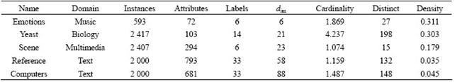
The details about the multi-label datasets are shown in Table 2, where the cardinality means the average number of labels assigned to the samples; the density denotes the average number of the ratio of sample labels to the total labels of the dataset; and the distinct denotes the number of different class label. The intrinsic dimension of the dataset denoted as d_im was exploited by the maximum likelihood estimator [17-18]. The above dataset could be downloaded from the following two web pages: http://mlkd.csd.auth.gr/multilabel.html (emotions, yeast and scene) and http://www.kecl.ntt.co.jp/as/ members/ueda/yahoo.tar.gz (reference, computers).

5.3 Evaluation metrics

Six evaluation metrics of multi-label dimensionality reduction are described as follows. Hamming loss (Ham. loss) computes the times that label-based prediction label is misclassified, and represents the average matching errors between the real labels and the predicted labels of testing samples. One-error evaluates the times of which the top-ranked label is not included in the set of relevant sample labels. Coverage denotes the distance to go down the ranked list of labels in order to cover all the relevant labels of the samples. Ranking loss (Rank. loss) expresses the number of times that irrelevant labels are ranked higher than relevant labels. Average precision (Ave. prec) evaluates the average fraction of labels ranked above a particular label and reflects the average accuracy of the predicted label samples in fact. Time reflects the time consumed by classification.

Table 1 Algorithm of MSDA

Table 2 Multi-label dataset and their statistics

5.4 Experiment results analysis

Tables 3-6 list the average (mean) and standard (STD) deviation of results after 100 iterations. From Tables 3-6, the experimental results on four multi-label datasets (emotions, yeast, scene and reference) are listed in the case that the original data are transformed to the intrinsic dimensions in the low-dimensional subspace. The intrinsic dimensionality is estimated by the forward MLE method. Note that “↓” indicates the smaller the better and “↑” indicates the larger the better. From Tables 3-6, it can be seen that the proposed MSDA algorithm is superior to ORI, PCA, LTSA, MLSI and MDDM on hamming loss, one-error, coverage, ranking loss, average precision and elapsed time. With regard to the average precision on five datasets, the result of MSDA is 4.25% higher than that of ORI, 16.15% than that of PCA, 12.88% than that of LTSA, 11.78% than that of MLSI, 3.50% than that of MDDM, and averagely 9.71% higher than that of other methods. In particular, PCA, LTSA and MLSI on the scene data do perform very poorly, which directly leads to serious deterioration of evaluation metrics and reflects the restrained limit of the three methods. The graph weighted matrix of samples features and similarity correlation matrix of partial labelled samples are employed together in MSDA, which makes it possible to preserve the intrinsic geometry structure of original high-dimensional data in satisfactory. Therefore, MSDA performs much better than unsupervised PCA, LTSA, MLSI and MDDM. MLSI, as a supervised algorithm, uses all the labelled samples, and does not exploit the latent relations among labels. And instead it only joins the simple matrix transformation. MDDM maximizes the independence between class labels and attributes and uses information provided by all the labelled samples. But in fact, the condition could not be satisfied, which is shown by the experiment results. It is the very advantageous point for the proposed semi- supervised dimensionality algorithm.

In order to compare the algorithms more clearly and visually, the results of the computers dataset are depicted by six sub-figures in Figs.1(a)-(f). From Figs.1(a)-(e), it is known that the rectangle bar of MSDA is lower than others, which shows that MSDA performs better than other methods as for the former four metrics. In Fig.1(e), the bar of MSDA is the highest, which expresses that MSDA has much higher average accuracy compared with other algorithms. Fig.1(f) represents the time elapsed by classifiers (e.g. MLKNN) after dimensionality reduction. It is obvious that the bar of MSDA is the shortest and MSDA spends the least time, which saves lots of valuable time.

Table 3 Results of emotions dataset (d_im=6, mean±STD)

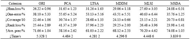
Table 4 Results of yeast dataset (d_im=21, mean±STD)

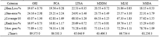
Table 5 Results of scene dataset (d_im=23, mean±STD)

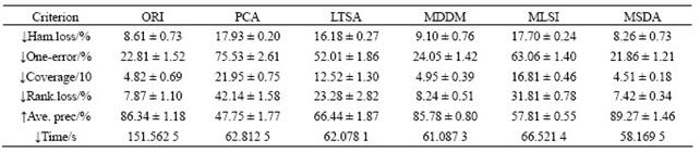
Table 6 Results of reference dataset (d_im=58, mean±STD)

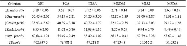
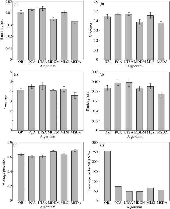
Fig.1 Comparison of different dimensionality reduction methods: (a) Hamming loss; (b) One-error; (c) Coverage; (d) Ranking loss; (e) Average precision; (f) Elapsed time

Figs.2 and 3 depict the performance curves of MSDA algorithm when labelled samples and the dimensions are different on the emotions dataset, respectively. Both of the two graphs show the influences caused by the several evaluation metrics all-together. And this further demonstrates that the number of labelled samples and different low-dimensions have influences on the performance of MSDA. It is easy to discover from Fig.2 that the performance of MSDA is ascending with the increase of labelled samples before the number of labelled ones reaches 0.50, in other words, using 0.30-0.50 labelled samples MSDA can achieve the same effects while using more labelled samples. MSDA would not improve any more when the number of labelled samples exceeds some thresholds. It can be seen from Fig.3 that it varies largely near the intrinsic dimension of the emotions dataset, before which the curve line is ascending quickly and after that the line becomes more gentle. This experimentally demonstrates that the approximate intrinsic dimensional dataset could preserve the intrinsic geometry structure of the original data  better. In addition, from the analysis of the above four datasets, PCA, LTSA and MLSI do not perform well on the scene dataset while they perform better on other datasets, which explains that there exists diversity to some extent when performing the same algorithm on different datasets. As a newly proposed semi-supervised dimensionality reduction algorithm especially for multi-label dataset, MSDA also has such a characteristic that would be influenced by different datasets.

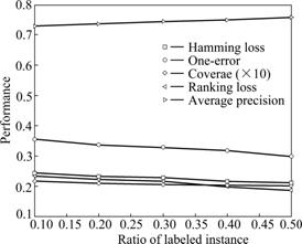
Fig.2 MSDA performance under different labeled samples with d_im=6

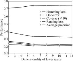
Fig.3 MSDA performance under different dimensions with d_im=6

6 Conclusions

(1) Aiming at dealing with the high-dimensional multi-label dataset in practical applications, a novel dimensionality reduction method called MSDA (multi- label dimensionality reduction based on semi-supervised discriminant analysis) is presented to reduce the dimensions. The method can preserve the intrinsic geometry structure of the original high-dimensional data in the low-dimensional sub-space. The average accuracy of multi-label classification using MSDA is 2.31%- 13.63% higher than those of other methods, and the remaining five performance evaluation metrics are also superior to other methods. In addition, MSDA saves a lot of time compared with ORI (the baseline), and the effectiveness of this method is validated.

(2) The combinations among semi-supervised learning, linear discriminant analysis and multi-label learning are embodied in MSDA. MSDA mainly focuses on efficiently employing the labelled and unlabeled samples to help better conduct dimensionality reduction on multi-label datasets. This introduced method provides a effective way to resolve the “curse of dimensionality” problem and the proposed novel idea is also very meaningful for the future researches or applications on dimensionality reduction of high-dimensional multi-label datasets.

References

[1] TSOUMAKAS G, KATAKIS I. Multi-label classification: An overview [J]. International Journal of Data Warehousing and Mining, 2007, 3(3): 1-13.

[2] LI Hong, LI Xiang, WU Min, CHENG Song-qiao, YI Li-jun. Multi-class classification of high-dimension gene expression profile based on closed patterns [J]. Journal of Central South University: Science and Technology, 2008, 39(5): 1035-1041. (in Chinese)

[3] van der MAATEN L J P. An introduction to dimensionality reduction using Matlab [R]. Maastricht: Maastricht University, 2007.

[4] CAI Deng, HE Xiao-fei, HAN Jia-wei. Semi-supervised discriminant analysis [C]// Proceedings of the 11th IEEE International Conference on Computer Vision. New York: IEEE Computer Society, 2007: 1-7.

[5] ZHU X J, GOLDBERG A B. Introduction to semi-supervised learning [J]. Synthesis Lectures on Artificial Intelligence and Machine Learning, 2009, 3(1): 1-130.

[6] ZHANG Dao-qiang, ZHOU Zhi-hua, CHEN Song-can. Semi-supervised dimensionality reduction [C]// Proceedings of the 7th SIAM International Conference on Data Mining. New York: IEEE Computer Society, 2007: 629-634.

[7] SONG Yang-qiu, NIE Fei-ping, ZHANG Chang-shui, XIANG Shi-ming. A unified framework for semi-supervised dimensionality reduction [J]. Pattern Recognition, 2008, 41(9): 2789-2799.

[8] CHENG H, HUA K A, VU K, LIU D Z. Semi-supervised dimensionality reduction in image feature space [C]// Proceedings of the 2008 ACM Symposium on Applied Computing. New York: ACM Press, 2008: 1207-1211.

[9] YU K, YU S P, TRESP V. Multi-label informed latent semantic indexing [C]// Proceedings of the 28th Annual International ACM SIGIR Conference on Research and Development in Information Retrieval. New York: ACM Press, 2005: 258-265.

[10] ZHANG Yin, ZHOU Zhi-hua. Multi-label dimensionality reduction via dependency maximization [C]// Proceedings of the 23rd AAAI Conference on Artificial Intelligence. New York: IEEE Computer Society, 2008: 1503-1505.

[11] PARK C, LEE M. On applying linear discriminant analysis for multi-labeled problems [J]. Pattern Recognition Letters, 2008, 29(7): 878-887.

[12] BOUTELL M R, LUO J B, SHEN X P, BROWN C M. Learning multi-label scene classification [J]. Pattern Recognition, 2004, 37(9): 1757-1771.

[13] GODBOLE S, SARAWAGI S. Discriminative methods for multi-labeled classification [C]// Proceedings of the 8th Pacific-Asia Conference on Knowledge Discovery and Data Mining (PAKDD). New York: IEEE Computer Society, 2004: 22-30.

[14] LIU Yi, JIN Rong, YANG Liu. Semi-supervised multi-label learning by constrained non-negative matrix factorization [C]// Proceedings of National Conference on Artificial Intelligence and Innovative Applications of Artificial Intelligence Conference. New York: IEEE Computer Society, 2006: 666-671.

[15] KANG F, JIN R, SUKTHANKAR R. Correlated label propagation with application to multi-label learning [C]// Proceedings of IEEE International Conference on Computer Vision and Pattern Recognition (CVPR). New York: IEEE Computer Society, 2006: 1719-1726.

[16] QI Guo-jun, HUA Xian-sheng, RUI Yong, TANG Jin-hui, MEI Tao, ZHANG Hong-jiang. Correlative multi-label video annotation [C]// Proceedings of the 15th International Conference on Multimedia. New York: ACM Press, 2007: 17-26.

[17] LEVINA E, BICKEL P J. Advances in neural information processing systems [M]. Cambridge: MIT Press, 2005: 777-784.

[18] FAN Ming-yu, QIAO Hong, ZHANG Bo. Intrinsic dimension estimation of manifolds by incising balls [J]. Pattern Recognition, 2009, 42(5): 780-787.

(Edited by LIU Hua-sen)

Corresponding author: LI Hong, PhD, Professor; Tel: +86-13975892566; E-mail: lihongcsu@mail.csu.edu.cn