J. Cent. South Univ. (2016) 23: 1468-1473

DOI: 10.1007/s11771-016-3199-5

Elimination of boundary effect for laminated overburden model in pillar stability analysis

ZHANG Peng(张鹏)^{1, 2}, K. A. Heasley²

1. Carlson Software, Watertown, MA 02472, USA;

2. Department of Mining Engineering, West Virginia University, WV 26505, USA

Central South University Press and Springer-Verlag Berlin Heidelberg 2016

Abstract: The laminated overburden model (LaModel) has been widely used for pillar design and stability analysis. As a boundary element program, the LaModel program is sensitive to the boundary condition, which should be considered before creating the model. To eliminate the boundary effect in a LaModel pillar stability analysis, a suitable boundary buffer zone is needed around the model edge. The radius of influence (R) and the abutment load extent (D) are two major factors that affect the stresses and displacements calculated in LaModel. To determine the optimum buffer zone extent, a database of case histories was analyzed using the LaModel program. Values for R and D were varied until a buffer zone having negligible influence on the pillar stability factor (SF) of the active mining zone (AMZ) was determined.

Key words: pillar stability; boundary effect; LaModel; numerical simulation; room-and-pillar

1 Introduction

In underground coal mines, the room-and-pillar mining method is widely used in flat, tabular deposits of thin seams, where rooms are cut into the coal bed leaving a series of coal pillars, to support the mine roof and control the flow of air. During retreat mining, pillars are partially or fully removed as secondary mining. Accurate analysis of the pillar stability is critical to mine design and mining activities.

Over the years, various versions of the analysis of retreat mining pillar stability (ARMPS) and the LaModel programs have been widely used in the U.S., and undoubtedly, they have improved the safety of room-and-pillar retreat mining operations [1]. To help to improve the underground safety of retreat mining in coal mines, the U.S. National Institute for Occupational Safety and Health (NIOSH) developed the ARMPS program [2]. The ARMPS program can model many standard retreat mining layouts and it is very accurate for “conventional” room-and-pillar retreat mining scenarios. However, it cannot be used in more complex, but ever more common situations, such as complex topography and multiple-seam interactions. On the other hand, the LaModel program is a numerical model that plays an important role in analyzing these complex mining scenarios [3-7].

Differing from ARMPS, an empirical based model, the LaModel program is based on the displacement- discontinuity (DD) variation of the boundary-element- method (BEM) with a laminated overburden. Different from other numerical modeling methods, such as finite element method (FEM), discrete element method (DEM) and finite difference method (FDM) [8-11], the overburden laminations in LaModel give the numerical model much more flexibility for stratified sedimentary geologies and multiple-seam mines. The overburden in LaModel is considered a stack of frictionless layers, and all of the layers are homogeneous having the same elastic modulus, Poisson ratio and thickness. LaModel is able to analyze large areas of single or multiple-seam coal mines, complex mining geometries, variable topography, and many other situations [12]. To improve LaModel’s performance in pillar design and stability analysis, a number of studies were conducted, such as calibrating the model based on field observation of deep cover and specific site conditions, and calculating the energy release in deep cover mining [13-15].

As a boundary element program, the LaModel program is sensitive to the boundary condition during the calculation of stresses and displacements. Further, its performance in pillar stability analysis can also be affected. Therefore, the boundary effect needs to be understood and considered when creating the model. In LaModel, instead of using “Rigid” boundary condition, the “Symmetric” boundary condition can be used to simulate a mirror image boundary without explicitly modeling the area outside the boundary of the model. In many single-seam cases, the “Symmetric” boundary condition can eliminate the boundary effect in pillar stability analysis.

However, it should be noted that when the area of interest is too close to the edge of the model, the boundary effect may still exist under the “Symmetric” boundary condition. To eliminate the boundary effect, the model needs to be large enough to ensure that the boundaries do not affect the area of interest in the model while not being overly large, thus increasing model run time. In this case, a sufficient buffer area is needed around the model edge. For the boundary buffer, it could be a solid pillar or a gob and its extent should be large enough that its influence can be neglected in pillar stability analysis. However, when the extent value is too large, the program will consume lots of time to run without improving its accuracy. Therefore, an optimum extent of the boundary buffer zone needs to be determined to eliminate the boundary effect in pillar stability analysis.

In LaModel, the radius of influence (R) and the abutment load extent (D) are two major factors that can be used as a reasonable extent for the boundary buffer zone. Both of these variables have primary effects on the calculation of stresses and displacements in the model. The radius of influence (R) is the extent of surface subsidence due to the seam convergence created by the extraction process, and it can be determined through the fundamental derivation of the laminated overburden model. The abutment load extent (D) is the extent of the abutment zone due to the adjacent gob, and it is also used in LaModel to calibrate the overburden to match that desired abutment extent.

In the following sections, the radius of influence (R) and the abutment load extent (D) are discussed in detail. Based on their values, several potential buffer zone extents are determined and applied to the database of case histories, and then their effect on the AMZ SF is investigated. Finally, their performances on eliminating the boundary effect are compared and the optimum value of the boundary buffer zone is determined.

2 Radius of influence

The frictionless laminated overburden model was originally introduced by Salamon and MUNRO [16] and then implemented into LaModel program by Heasley [17]. The laminated overburden model is based on the thin plate theory and the formulations assuming that the displacements and stresses are continuous across the layers. The overburden in LaModel consists of a stack of strata laminations where the interfaces between beds are all horizontal and free of shear stresses and cohesion (see Fig. 1).

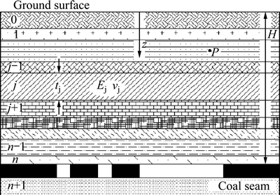
Fig. 1 Schematic of laminated overburden [17]

Derived from the laminated overburden model, the vertical displacement (W) at (x, y) due to a unit element convergence (1.0) at seam level (z) can be presented as

                              (1)

where λ is a factor related to the lamination thickness (t) and Poisson ratio (v) of the laminated overburden, which is shown as

                                   (2)

In the laminated overburden model, the seam and overburden are considered to be infinite media. Therefore, in order to achieve the entire surface displacement caused by a unit element convergence (1.0), the unlimited extension planar of s[-∞, +∞] is used for the integral:

 (3)

For this integral case, it can be simplified and solved by transforming from the Cartesian coordinate system to the polar coordinate system:

                 (4)

When the radius of influence (R) tends to +∞, the entire surface displacement induced by a unit seam convergence at the seam level (z) can be obtained. Meanwhile, a certain percentage (p) of the entire surface displacement could be determined as

                 (5)

In reality, the dimensions of a numerical model cannot tend to +∞ during the development of the model. However, the numerical model can be created with a dimension (R) where a certain percentage (p) of the entire surface displacement is included in this area. In that case, the radius of influence (R) can be derived and used as the extent of the boundary buffer zone:

                              (6)

where R is the radius of influence; p is the desired percentage of surface convergence, in decimal; t is the lamination thickness; v is the Poisson ratio of laminations; z is the depth.

To obtain sufficient significant digits and accuracy in the numerical calculation of the laminated overburden model, the desired percentage (p) is set as 99.9999% in this research. In the following section, the equivalent radius of influence (R) is used as the extent of boundary buffer zone to analyze its performance on eliminating the boundary effect on LaModel.

3 Abutment load extent

In underground coal mines, there are often loads on the pillars due to the adjacent areas of pillar retreat mining, including side abutment loads and front abutment loads. Figure 2 shows the front abutment loads applied to the pillars within the active mining zone (AMZ) during extraction [2].

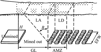
Fig. 2 Schematic of applied loads on AMZ [2] (AMZ: Active mining zone; H: Depth of cover; B: Abutment angle; LA: Abutment load; EFW: Extraction front width; LD: Development load; GL-Mined out area)

The magnitude of the abutment load is commonly conceptualized and calculated using the “Abutment Angle” concept. This concept is based on the abutment load estimation in the analysis of longwall pillar stability (ALPS), which is widely used for longwall pillar design [2, 18-19]. Figure 3 shows two typical conditions of the “abutment angle” concept (supercritical and subcritical), where the total abutment load is considered to be the weight of the wedge of overburden defined by a vertical line at the edge of the panel and the line at the “abutment angle” (β) on the inside of the panel. The weight of the overburden within the abutment angle wedge is supported by the pillars and, as a corollary, the gob is assumed to support the remainder of the overburden weight over the full-extraction area. Using field measurements of abutment loading, a suitable average abutment angle for use in the United States was determined to be 21° [18].

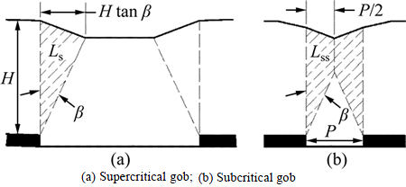
Fig. 3 Schematic of abutment angle [20]:

There are two types of panels based on their relative dimensions (see Fig. 3). A “supercritical” panel is wide enough that the abutment angle lines do not cross before they intersect the surface. Therefore, from geometry, the panel width (P) is greater than twice the distance of the abutment angle intercept on the surface, which is equal to the depth (H) times the tangent of the abutment angle (β). For a supercritical panel, knowing the density of the overburden (δ_r), the magnitude of the abutment load (L_s) for a supercritical panel can be calculated from the geometry:

                             (7)

A “subcritical” panel is defined as a panel that is narrow enough that the abutment angle lines cross before they intersect the surface. Therefore, from geometry, the width (P) of a subcritical panel is less than twice the depth times the tangent of abutment angle (β). Based on the geometry, the abutment load for a subcritical panel (L_ss) can be calculated:

                      (8)

The abutment load stress distribution (σ_a) was found to be a square decay relationship given in Eq. (9) and it is related to the magnitude of the abutment load (L_s) and the distance from the edge of the panel (x).

                       (9)

Based on Eq. (9), the abutment load distribution can be determined and plotted in Fig. 4, which shows the distribution of side abutment load stress. It indicates that the peak abutment stress at the edge of the panel (x=0) is equal to 3L_s/D and then it decreases as a squared function of the distance from the edge of the panel until the stress reaches zero at a distance of D.

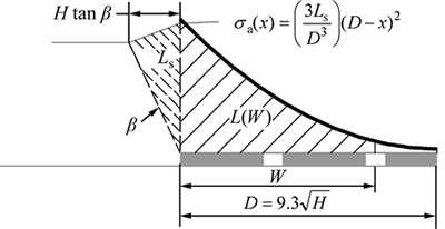
Fig. 4 Schematic of side abutment load distribution extent [21]

Mark [19] analyzed the stress distribution of the abutment load (L) based on field measurements of the side abutment load. It was found that the maximum extent of the abutment load (D) was a function of the depth (H):

                                 (10)

And 90% of the abutment load falls within a distance of which is presented in Eq. (11). It should be noted the depth (H) in Eqs. (10) and (11) needs to be in units of feet.

                                   (11)

Figure 5 shows the schematic of the front abutment load distribution based on filed observations [2], which indicates that the maximum extent of front abutment load has an extent of and 90% of the load is within a range of

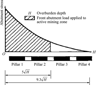
Fig. 5 Distribution of front abutment load [2]

When the abutment load extent is determined through field observation at a given site, it can be used to calibrate the lamination thickness of the overburden to match that abutment extent in LaModel through the following equation [13]:

                      (12)

where E is the elastic modulus of overburden; v is the Poisson ratio of overburden; E_s is the elastic modulus of seam; h is the seam thickness; D_n is the abutment load extent; n is the percentage of abutment load.

When the field observation is not available or too difficult to obtain, the empirically suggested extent of (contains 90% of front abutment load, see Fig. 5) is often considered to be the “practical” extent of the abutment load [2] and used in LaModel to calibrate the overburden [13]. experience has shown that the pillars within this range typically behave as a system and is also employed as the breadth of the AMZ used in ARMPS and LaModel programs in pillar design [2, 13].

For the abutment load extent, theand are based on field experience and they may vary from case to case. Therefore, in the following section, five different values (and) were used as the extent of the boundary buffer zone and their performance on eliminating the boundary effect was investigated.

4 Case history database

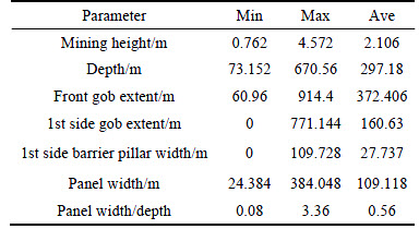
To investigate the influence of the boundary buffer extent on the accuracy of pillar stability analysis, a subset of the most current ARMPS database was used. This subset database consists of 50 case histories which belong to the third loading condition in ARMPS. It means that their mine plans contain an active gob and one side gob. Additionally, the 50 case histories were selected in such a way that the range of input parameters matched the range of values observed in the ARMPS database. Table 1 lists the geometric ranges of the 50 case histories. The mining height ranges from 0.762 to 4.572 m (2.5 to 15.0 ft) with an average value of 2.106 m (6.91 ft); the depth ranges from 73.152 to 670.560 m (240 to 2200 ft) with an average value of 297.18 m (975 ft), the active gob extent ranges from 60.960 to 914.400 m (200 to 3000 ft) with an average value of 372.406 m (897 ft); the 1st side gob ranges from 0.0 to 771.144 m (0.0 to 2530 ft) with an average value of 160.63 m (527 ft); the 1st side barrier pillar width ranges from 0.0 to 0.0 to 109.728 m (360 ft) with an average value of 27.737 m (91 ft); the panel width ranges from 24.384 to 384.048 m (80 to 1260 ft) with an average value of 109.118 m (358 ft); and the panel width-to- depth ratio ranges from 0.08 to 3.36 with an average value of 0.56.

Table 1 Mine geometry ranges of selected fifty case histories

5 Optimum extent of boundary buffer zone

Based on the 50-case history database, the radii of influence (R), and were used as the extent of the boundary buffer zone in each numerical model. Since the stability factor (SF) of AMZ is normally used in pillar design and stability analyses [2, 21-22], the numerical simulation results using different boundary buffer zone were analyzed based on the calculated AMZ SF.

The value of AMZ SF is determined by comparing the load bearing capacity of the pillars in the AMZ against the loads applied to those pillars [2]. In a recent research effort, a computer code of ARMPS-LAM was developed to effectively implement the laminated overburden model into the ARMPS program [23]. The ARMPS-LAM program takes the basic ARMPS geometric input for defining the mine plan and loading condition, and then automatically develops, runs and analyzes a full 3D LaModel analysis to calculate and output the AMZ SF. Since it can also run in batch mode, the AMZ SF of each model can be quickly obtained when the extent of the boundary buffer zone is specified.

To compare the numerical calculation accuracy with different buffer zone extents, the AMZ SF error (absolute difference in AMZ SF) was investigated. In this research, the calculated AMZ SF using the widest extent available,as the boundary buffer zone was selected as the most accurate or “Base” value. Then, the absolute difference of the AMZ SF values between the various buffer distances was used as the AMZ SF error. Finally, after running the 50 case histories with different boundary buffer zone extents, the average values and standard deviations of the AMZ SF error were determined and shown in Table 2.

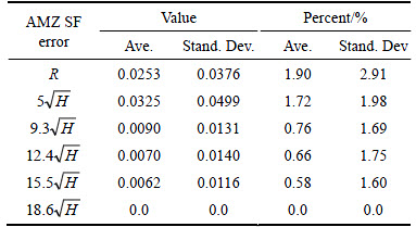
Table 2 shows that when the boundary buffer zone is R,and the average AMZ SF errors are 0.0253 (1.90%), 0.0325(1.72%), 0.0090 (0.76%), 0.0070 (0.66%) and 0.0062 (0.58%), respectively. Note that when was used as the boundary buffer zone, the AMZ SF error is the highest one among these different sizes. The radius of influence (R) is more accurate than and less accurate than When the buffer zone extent increases from to the accuracy of AMZ SF is increasing as well.

Table 2 Comparison of AMZ SF error with different boundary buffer zones

However, it should be noted that in room-and-pillar mine design, the AMZ SF generally has an apparent accuracy of two decimal places. In that case, if the AMZ SF error is less than 0.005, the changes in the buffer zone size will not “significantly” affect the results of AMZ SF calculation. Therefore, an optimum value of the boundary buffer zone should meet the AMZ SF accuracy requirement, i.e., AMZ SF error <0.005. The AMZ SF accuracy requirement is highlighted by a red dash line in Fig. 6.

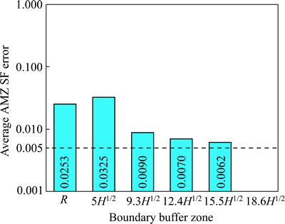
Fig. 6 Average AMZ SF error vs boundary pillar size

Although the accuracy increases as the buffer zone size increases, none of them quite meet the AMZ SF desired accuracy requirement of 0.005 (although it gets very close). Ultimately, based on the analysis above, was selected as the optimum value of the boundary buffer zone, where the stress influence has a practically negligible boundary effect on the AMZ SF and pillar stability analysis.

6 Conclusions

1) The radius of influence (R) of the laminated overburden model is derived based on the equation of surface displacement induced by the convergence of a unit seam element.

2) The abutment loads for supercritical and subcritical panels are determined based on the “abutment angle” concept. The abutment load stress distribution is related to the magnitude of the abutment load and the distance from the edge of the panel.

3) Based on the radius of influence (R) and abutment load extent (D), several potential buffer zone extents were applied to a database with 50 case histories. And their calculated AMZ SFs were used to investigate their influence on pillar stability analysis. It is found that the results accuracy is proportional to the extent of buffer zone.

4) Based on the comparison results of potential buffer zone extents, the is selected as the optimum value of boundary buffer zone, where the stress influence has a practically negligible boundary effect on the AMZ SF and pillar stability analysis. It should be noted that the depth (H) needs to be in units of feet.

References

[1] TULU I B, HEASLEY K A, MARK C. A comparison of the overburden loading in ARMPS and LaModel [C]// Proceedings of the 29th International Conference on Ground Control in Mining. Morgantown: West Virginia University, 2010: 28-37.

[2] MARK C, CHASE F E. Analysis of retreat mining pillar stability (ARMPS) [C]// Proceedings of the New Technology for Ground Control in Retreat Mining. Pittsburgh: NIOSH, 1997: 17-34.

[3] AKINKUGBE O, HEASLEY K A. The new two-dimension LaModel program [C]// Proceedings of the 23nd International Conference on Ground Control in Mining. Morgantown: West Virginia University, 2004: 146-153.

[4] CHASE F E, WORLEY P, MARK C. Multiple seam mining interactions: case histories from the Harris No. 1 mine [C]// Proceedings of the 24th International Conference on Ground Control in Mining. Morgantown: West Virginia University, 2005: 79-86.

[5] HEASLEY K. LaModel analysis of the crandall canyon mine collapse [C]// Proceedings of the 43rd US Rock Mechanics Symposium & 4th US–Canada Rock Mechanics Symposium. Asheville: American Rock Mechanics Association, 2009.

[6] HEASLEY K A, AGIOUTANTIS Z. LAMODEL—A boundary element program for coal mine design [C]// Proceedings of the 10th International Conference on Computer Methods and Advances in Geomechanics. Brookfield: Balkema, 2001: 9-12.

[7] HEASLEY K A, CHEKAN G J. Practical boundary-element modeling for mine planning [C]// Proceedings of the 2nd International Workshop on Coal Pillar Mechanics and Design. Pittsburgh: NIOSH, 1999: 73-87.

[8] MURALI M G, SHEOREY P, KUSHWAHA A. Numerical estimation of pillar strength in coal mines [J]. International Journal of Rock Mechanics and Mining Sciences, 2001, 38(8): 1185-1192.

[9] DENG J, YUE Z, THAM L, ZHU H. Pillar design by combining finite element methods, neural networks and reliability: a case study of the Fenghuangshan copper mine, China [J]. International Journal of Rock Mechanics and Mining Sciences, 2003, 40(4): 585-599.

[10] ESTERHUIZEN E, MARK C, MURPHY M M. Numerical model calibration for simulating coal pillars, gob and overburden response [C]// Proceedings of the 29th International Conference on Ground Control in Mining. Morgantown: West Virginia University, 2010: 46-57.

[11] LI C, XU J, WANG Z, QIN S. Domino instability effect of surrounding rock-coal pillars in a room-and-pillar gob [J]. International Journal of Mining Science and Technology, 2013, 23(6): 913-918.

[12] WANG Q, HEASLEY K. Stability mapping system [C]// Proceedings of the 24th International Conference on Ground Control in Mining. Morgantown: West Virginia University, 2005: 243-249.

[13] HEASLEY K A. Some thoughts on calibrating LaModel [C]// Proceedings of the 27th International Conference on Ground Control in Mining. Morgantown: West Virginia University, 2008: 7-13.

[14] HEASLEY K A, SEARS M M, TULU I B, CALDERON-ARTEAGA C H, JIMISON II L W. Calibrating the LaModel program for deep cover pillar retreat coal mining [C]// Proceedings of the 3rd International Workshop on Coal Pillar Mechanics and Design. Morgantown: West Virginia University, 2010: 47-57.

[15] SEARS M M, HEASLEY K A. An Application of Energy Release Rate [C]// Proceedings of the 28th International Conference on Ground Control in Mining. Morgantown: West Virginia University, 2009: 10-16.

[16] SALAMON M D G, MUNRO A H. A study of the strength of coal pillars [J]. Journal of the South African Institute of Mining and Metallurgy, 1967, 68(2): 55-67.

[17] HEASLEY K A. Numerical modeling of coal mines with a laminated displacement-discontinuity code [D]. Golden: Colorado School of Mines, 1998.

[18] MARK C. Pillar design methods for longwall mining [M]. Pittsburgh, US: Department of the Interior, Bureau of Mines, 1990.

[19] MARK C. Analysis of longwall pillar stability (ALPS): an update [C]// Proceedings of the Workshop on Coal Pillar Mechanics and Design. Pittsburgh: US Department of the Interior, Bureau of Mines, 1992: 238-249.

[20] MARK C, GAUNA M, CYBULSKI J, KARABIN G. Applications of ARMPS (version 6) to practical pillar design problems [C]// Proceedings of the 30th International Conference on Ground Control in Mining. Morgantown: West Virginia University, 2011.

[21] BISE C J. Modern American coal mining: Methods and applications [M]. Englewood: Society for Mining, Metallurgy, and Exploration, 2013.

[22] GHASEMI E, ATAEI M, SHAHRIAR K. Prediction of global stability in room and pillar coal mines [J]. Natural Hazards, 2014, 72(2): 405-422.

[23] ZHANG P, HEASLEY K A. Initial results from implementing a laminated overburden model into ARMPS [C]// Proceedings of the 32nd International Conference on Ground Control in Mining. Morgantown, WV: West Virginia University, 2013: 239-247.

(Edited by YANG Hua)

Received date: 2015-02-04; Accepted date: 2015-06-11

Corresponding author: ZHANG Peng, PhD, Engineer; Tel: +1-617-3932300; E-mail: pzhang@carlsonsw.com