Two-dimensional cellular automaton model for simulating structural evolution of binary alloys during solidification

ZHANG Lin(张 林), ZHANG Cai-bei(张彩碚)

School of Science, Northeastern University, Shenyang 110004, China

Abstract: Two-dimensional cellular automaton(CA) simulations of phase transformations of binary alloys during solidification were reported. The modelling incorporates local concentration and heat changes into a nucleation or growth function, which is utilized by the automaton in a probabilistic fashion. These simulations may provide an efficient method of discovering how the physical processes involved in solidification processes dynamically progress and how they interact with each other during solidification. The simulated results show that the final morphology during solidification is related with the cooling conditions. The established model can be used to evaluate the phase transformation of binary alloys during solidification.

Key words: binary alloys; phase transformation; solidification; diffusion; nucleation; computer simulation; cellular automaton

1 Introduction

During solidification of cast metallic materials, simulations of microstructural evolution, which track kinetics in a local fashion, are of interest for two reasons. First, from a fundamental point of view, it is desirable to better understand the dynamics and the topology of microstructures that arise from the interaction of large number of lattice defects. Second, from a practical point of view, it is necessary to predict microstructure parameters such as grain size or texture which determine the mechanical and physical properties of as-solidified materials subjected to industrial processes[1]. During the past decades, the modelling of solidifying systems has been an active and engrossing field of study. A number of excellent models for discretely simulating dendrite growth have been suggested. They can be grouped as phase field models[2,3], Monte Carlo models[4,5] and cellular automaton models[6-10].

Complementary to these approaches, a cellular automation(CA) model is introduced to simulate the structural evolution of solidifying grains during phase transformations of binary alloys. During the phase transformation of the above chosen binary alloys, nucleation, growth of nucleated grains and mass-heat transfer in solid and liquid phases are involved in the model. In modelling the phase transformation, the diffusion kinetics is calculated using an explicit finite volume technique[11], and the local concentration and heat changes are incorporated into a nucleation or growth function which is utilized by the automaton in a probabilistic fashion.

2.1 Basic assumptions

The model involves the following assumptions. First, homogeneous nucleation takes place in liquid. Second, the effect of convection on the changes of solute and temperature fields is not taken into account. Third, the modelling does not account for the transformation from solid to liquid. Fourth, for the binary alloy with a certain concentration, the transformation temperature from liquid to solid is the temperature on the liquidus of the phase diagram of the binary alloy corresponding to this concentration.

2.2 Mathematical formulation

The phase transformation by cooling can be described as Liquid→Liquid+α, where Liquid denotes the liquid phase and α the solid phase. Precipitation of the second solid phase β from the first solid phase α, α→α+β, will be arisen by cooling below the β solves as shown in Fig.1.

Fig.1 Schematic phase diagram of Sn-Pb binary alloy (Liquid  represetns liquid phase, α is first solid phase, and β is second solid phase)

A continuous nucleation distribution dn/d(ΔT′) at an undercooling  can be written in

     (1)

              (2)

where  ΔT_max is the mean undercooling,  standard deviation, n_max total area[6], and f_s is the fraction of solid already formed.

The diffusion processes of both mass (solute) and heat can be described by

                             (3)

                              (4)

where  t is time, C_υ is a solute concentration in phase υ (liquid l or solid s), D_υ is the associated diffusion constant, and D_u is a temperature field diffusion constant. u characterizes a dimensionless temperature field[12], which is the thermal supersaturation and can be expressed by the relation

                          (5)

Growth of either columnar or equiaxed grains can be calculated with the aid of the LGK model[13]:

                   (6)

                                  (7)

                 (8)

-D_cG_c=vG_l(1－k)                             (9)

                               (10)

                                (11)

where  Pe is the solute Péclet number of the dendrite tip, k=C_s/C_l is a solute partition coefficient at the interface, E(Pe) is a exponential integral, C₀ is the composition of the modelled alloy, R is the radius of dendrite tip, υ is the instantaneous velocity of dendritic tip, Γ is the Gibbs-Thomson coefficient, m is the slope of the liquidus (it can be determined by calculating the tangent slope along the liquidus at the different solute concentrations), G is the thermal gradient, ξ_c is a function of the Péclet number, P_u­ is the thermal Péclet number of the dendrite tip, and G_c is the associated solute gradient in liquid at the tip.

A cellular automaton is a dynamical system, in which space, time, and states of the system are discrete. Each cell in the regular spatial lattice can be in any one of a finite number of states. The rules of transition, which determine the evolution of a given cell during one time step, are defined according to the states of its neighbor cells[14].

Fig.2 is a schematic representation of this CA lattice with a two-dimensional 200×200 square enmeshment of cells. Hence, the simulated results could be interpreted as what happens in a cross-section of the simulated grains. The neighbors of one cell are defined as the Moore neighborhood as shown in Fig.3. Two boundary conditions are presented in this modelling. First, as a schematic network of cells in a regular lattice arrangement shown in Fig.4, the bottom of the network is assumed to be next to the mould. The network is cut properly by two planes perpendicular to the mould surface and periodic conditions are set on these two boundary planes (the dot lines shown in Fig.4). The network is symmetric about its top. Second, periodic boundary condition at each boundary face is also used in the simulation.

The state attributes of each cell are characterized by the following parameters: the state identifier (solid, liquid/solid interface or L/S interface, and liquid as shown in Fig.2), the cell index (0 for liquid and each of 1-100 for a possible grain crystallographic orientation), the growth length, solute mass fraction (taking its real value of 0.0-1.0), and temperature field. The CA lattice is undercooled at a given cooling rate .

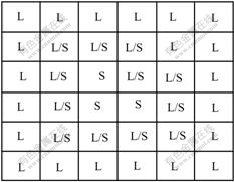
Fig.2 Schematic illustration of ‘S/L interface’ cells which separate S and L domains corresponding to three states (‘S/L interface’, Solid and Liquid) of cells in CA lattice

Fig.3 Cell lattice used in model(Labels 1-8 are neighbor cells of cell C)

Fig.4 Schematics for cellular automaton in a volume

At the beginning of the simulation, each cell is set to liquid with the same initial solute content, i.e. the composition of the alloy C₀, and the same initial temperature T₀, which is a little higher than the liquidus T_fre of the simulated alloy on its phase diagram, corresponding to the composition of the specimen. The decreasing of the temperature T_∞ of the CA lattice is written as T_∞→T_∞－, where τ is a time step, and the temperature of each cell is given by the following Eqn.(19) after local temperature changes are evaluated. When the temperature is decreased to below the transformed temperature of β phase, the left liquid phase cells are transformed into β phase.

According to Eqn.(2), the density increase, δn_v or δn_s, of new nuclei nucleated within the volume of the melt or on the mould surface at the undercooling temperature increases by an amount δ(ΔT)[δ(ΔT)>0] during one time step τ, is given by

          (12)

where  f_s takes the following value

                     (13)

 and  denote the solute concentrations which can be determined by the liquidus and solidus of the studied alloy as shown in Fig.1. The nucleation probability, p_v or p_s, during solidification is given by

p_v=δn_vV  or  p_s=δn_sS                        (14)

where V represents the volume of one cell, and  the surface area of one mold cell. In the simulation, each untransformed cell to solid with a generated random number r(≤r＜1) in the volume or on the surface of the specimen is scanned. If r≤p_v or r≤p_s to the untransformed cell, this cell will nucleate.

3.2 Solute and temperature redistribution

For a solidified cell (i, j), the increase of the temperature field is given by

u_(i,j)→u_(i,j)＋l_a?f_s,(i,j)                                         (15)

where  l_a is a dimensionless latent heat.

For a liquid cell (m, p) near the solidified cells like the cell (i, j), the increased amount of solute is expressed as

C_(m,p)→C_(m,p)+C_reject                         (16)

                   (17)

where  C_(m,p) is the solute concentration of the liquid cell (m, p) before receiving the rejected solutes from its neighbor solidified cells, C_reject is the total amount of rejected solute concentration from all the solidified cells near the cell (m, p), hence (C_(i,j)－) is the

concentration difference of the cell (i, j) before and after solidification. The summation covers all kinds of solidified cells contributing to the cell (m, p). Once the liquid cell (m, p) receives solutes from the solidified cells, the ‘S/L interface’ cell is produced, which is located between any solid and liquid cells. Hence, solutes are enriched in this ‘S/L interface’ cell. When there is enough time of solute diffusion, the enriched solutes can be diffused into neighboring cells, and crystal can grow steadily. However, if crystal grows very quickly, these enriched solutes have no time to diffuse, and the growing interface of crystal will become unsteady.

In the diffusion calculations including solute and the temperature field, the central differentials of Eqn.(3) and Eqn.(4) take the following forms to reduce the influence of diffusion anisotropy from the cubic cell lattice chosen in the model. The change of temperature field of one cell (i, j), as shown in Fig.5, during one time step τ due to diffusion can be calculated in the following way:

    (18)

Fig,5 Discretized diffusion operator of cell (i,j)  with its nearest (1-8) neighbors

where  ξ₀ is the distance between two adjacent grid points. Then, the temperature of the cell (i, j) after τ can be given as follows:

T_(i,j)=T_∞＋L?u_(i,j)/C_p                                         (19)

The calculation of solute diffusion is rather more complex than that of temperature field diffusion:

(20)

Case A: If the cell (i, j) with its one neighbor cell ‘nei’ is in the same phase υ,

χ_nei,(i,j)=χ_(i,j)=D_υ                              (21)

where  χ_{nei, (i,j)} is used to represent the coefficient from χ_(i,j-1) to χ_(i-1,j+1) in Eqn.(21) corresponding respectively to the eight neighbors of the cell (i, j), as shown in Fig.5.

Case B: If the cell (i, j) belongs to the phase υ, whereas its one neighbor cell ‘nei’  belongs to the interface,

  and χ_(i,j)=D_υ  (22)

Case C: If both the cell (i, j) and its one neighbor cell ‘nei’ belongs to the interface,

                    (23)

with .  f_s(i,j) or f_s,nei,(i,j) is calculated by

or             (24)

where  or  ( or ) is the concentration of the cell (i, j) (its one neighbor cell) on the liquidus or solidus of the phase diagram at the temperature T_{(i, j)} (T_{nei, (i, j)}).

3.3 Grain growth

After a cell has been solidified at a certain time t₀, the cell grows towards its neighbor ‘S/L interface’ cells. The growing length ξ_d (t) is calculated by an integral over the time of growth for the dendrite tip. Here, d=1-8, presents respectively the eight directions from one cell  (i, j) towards its neighbors as shown in Fig.3, and ξ_d (t) can be written as

                             (25)

where  v_d indicates an instantaneous growth velocity to the d th neighbor of eight neighbors from the cell (i, j). The capture probability p_d to the neighbor ‘S/L interface’ cell along the d th direction of this solid cell can be given by

                              (26)

Hence, to a ‘S/L interface’ cell ‘nei’, if its temperature T is lower than its T_fre, corresponding to its solute concentration, and its generated ‘transformed’ probability r_tra (0≤r_tra＜1) is smaller than a ‘capture’ probability p_d of its neighbor solid cell (i, j) towards the cell ‘nei’, the cell ‘nei’  will become solid.

3.5 Time step

The time step τ is one key measure in the modelling because the state of each cell is changed rhythmically with its increase, and it could be defined as

                (27)

where  v _max is the maximum growth velocity among the growth velocities for all solid cells and ‘min’ means the minimum value of four items in the round bracket.

The microstructural evolution of small specimens with the size of 2 mm×2 mm is simulated by the present CA model. Fig.6 and Fig.7 adopt the boundary condition as shown in Fig.4, and Fig.8 shows the periodic boundary condition. In these simulated pictures, liquid cells and other different grains are represented by different grey scales.

Fig.6 shows the morphologies of a Ni-20%Cu(mass fraction) alloy from the beginning temperature of 1 410 ℃ to 1 406 ℃ at various cooling rates, in which (a) is for the cooling rate of 0.1 ℃/s, (b) for 0.05 ℃/s, and (c) for 0.01 ℃/s. In these figures, nucleation is caused only on the mould surface but not in the bulk for the higher probability on the mould surface than that in the bulk. Growth of the columnar grains originated from the mould wall towards the bulk depends obviously on the cooling rates, and it is an example of diffusion-controlled growth. If the cooling rate is reasonably small (for example, 0.01 ℃/s in Fig.6(c)), the time interval needed to reach the temperature of 1 406 ℃ is properly long. Hence there is more time to make the diffusion processes of solute and temperature fully go on, and a solute (and temperature) distribution preferable to growth of grains could be produced. Therefore, the final columnar grains with 1 406 ℃ become longer for a properly smaller cooling rate such as 0.01 ℃/s in Fig.6(c) than for a quicker one such as 0.1 ℃/s in Fig.6(a).

Fig.7 shows the simulated microstructures of Ni-20%Cu(mass fraction) alloy respectively at 0.08 ℃/s in Fig.7(a) and Fig.7(b) and at 0.03 ℃/s in Fig.7(c) and Fig.7(d) with the temperatures θ₂=1 383 ℃ and θ₃=1 340 ℃. The comparison between two structures at the same temperature but different cooling rates gives an insight into how the cooling conditions affect the grain morphologies. The transition from columnar grains to equiaxed grains(TCE) could take place if the difference between the temperature (θ₁, or θ₂) and the melting point is higher than ΔT_v,max. It can be seen from Fig.7 that the equiaxed grains can form before the columnar grains extend to larger region, and the trend is more pronounced when the cooling rate is larger (0.08 ℃/s as shown in Fig.7(a)).

This phenomenon can be explained as follows. As described above, each liquid cell in the melt bulk and on the mould with an undercooling temperature is a potential nucleation site. By cooling, the nucleation probability becomes large for each potential nucleation site, and it means that those cells may nucleate. Nevertheless, the nucleated cells will push an amount of solutes into their neighbor liquid cells and release certain latent heat. Then, the concentrations of the liquid cells

Fig.6 Grain growth of Ni-Cu20% alloy at different cooling rates to final temperature θ=1 406 ℃ from beginning temperature of   1 410 ℃: (a) 0.1 ℃/s; (b) 0.05 ℃/s; (c) 0.02 ℃/s

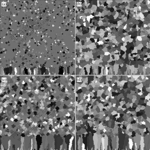
Fig.7 Microstructures with θ₂=1 383 ℃ and θ₃=1 340 ℃ respectively: (a) and (b) at 0.08 ℃/s; (c) and (d) at 0.03 ℃/s

neighboring to the solidified grains become enriched, and their temperatures become high resulting from the temperature field diffusion. These lead to the fact that the undercooling temperatures (ΔT=T_fre－T) of these cells vary from their starting values and their nucleation probability will vary. In addition, the diffusion procedures of solute and temperature will start from other liquid cells not those neighboring to the solid cells, and they will also lead to the variances of undercooling temperatures to these liquid cells. Therefore, nucleation of liquid cells both neighboring and not neighboring to solid cells is controlled by diffusion. Growth of those solid cells will be caused if there exist undercooling temperatures in their neighboring untransformed cells and concentration and temperature differences between a solid cell and its neighboring untransformed cells, and it is also a diffusion-controlled procedure. Thus, on one hand, the nucleation probability or number of liquid cells is smaller for a lower cooling rate than that for a quicker one. On the other hand, at such a low cooling rate, because the diffusion can continue for a longer time, or more sufficient performance can be obtained, than at a quicker one, it yields a more uniform distribution of solute and temperature around each solidified cell, and leads to a larger equiaxed grains being generated as shown in Fig.7(d) for θ=1 340 ℃.

Figs.8(a) and (b) demonstrate the evolution of metallurgical structure for a low composition eutectic alloy of Pb-5%Sn(mass fraction) at different temperatures for θ₁=320℃, and θ₃=80 ℃ respectively at the cooling rate =0.15 ℃/s. In the beginning, a few grains nucleate in the liquid bulk. Then, as the temperature decreases, the nucleated grains begin to grow and more and more grains nucleate (as shown in Fig.8(a)). Finally, Fig.8(b) displays the morphology with many large and small grains. Fig.8(b) attracts one’s attention to fine spread β phases which precipitate from the bulk phases α as dots or stripes. It could come from that a little of liquid is left and embedded in them. When the temperature of the alloy is decreased below the solidus of β phase, the precipitation of β phases occurs immediately.

Fig.8 Evolution of metallurgical structure and phase transformations of low concentration eutectic alloy Pb-5%Sn with different temperatures for θ₁=320 ℃(a) and θ₃=80 ℃(b) at cooling rate 0.15 ℃/s (Precipitation phase β spreads in bulk phase α as dots and stripes ( in white squares □))

1) Nucleation of grains is mainly determined by two factors. First, there are undercooling temperatures on those potential nucleation sites; second, on those sites, nucleation probabilities must be large.

2) The phase transformation from liquid to solid owing to growth of grains is determined by the following factors. First, there are undercooling temperatures on those liquid cells; second, they are neighboring upon solid cells; third, probabilities that those solid cells ‘capture’ those neighboring liquid cells must be large.

3) For the same initial composition of alloy, the final morphology during solidification, for example the average size of grains, is related to the cooling rate chosen. Reasonably cooling rate is useful to acquire a desired morphology of alloy.

References

[1] RAABE D. Introduction of a scalable three-dimensional cellular automaton with a probabilistic switching rule for the discrete mesoscale simulation of recrystallization phenomena [J]. Philo Mag A, 1999, 79: 2339-2358.

[2] ZHANG Y T, LI D, LI Y, PANG W. Numerical simulations of equiaxed dendrite growth using phase field method [J]. J Mater Sci Technol, 2002, 18: 51-53.

[3] ZHAO D P, JING T, LIU B C. Simulating the three- dimensional dendritic growth of Al alloy using the phase-filed method [J]. Acta Phys Sin, 2003, 52: 1737-1342. (in Chinese)

[4] GUO J Y, HONG Z K, CHEN M, GUN Z Y. A Monte Carlo simulation on solidification and crystal growth of metals [J]. J Engineering Thermophysics, 2001, 22: 725-728. (in Chinese)

[5] ZHU P, SMITH R W. Dynamic simulation of crystal growth by Monte Carlo method [J]. Acta Metall Mater, 1992, 40: 3369-3379.

[6] RAPPAZ M, GANDIN C A. Probabilistic modelling of micro- structure formation in solidification processes [J]. Acta Metall Meter, 1993, 41: 345-360.

[7] ZHANG L, ZHANG C B, LIU X H, WANG G D, WANG Y M. Modeling recrystallization of austenite for C-Mn steels during hot deformation by cellular automaton [J]. J Mater Sci Tech, 2002, 18: 163-166.

[8] ZHANG L, WANG Y M, ZHANG C B, WANG S Q, YE H Q. A cellular automaton model of the transformation from austenite in low carbon steels [J]. Modelling Simul Mater Sci Tech, 2003, 11: 791-801.

[9] ZHANG L, ZHANG C B, WANG Y M, WANG S Q, YE H Q. A cellular automaton investigation of the transformation from austenite to ferrite during continuous cooling [J]. Acta Mater, 2003, 51: 5519- 5527.

[10] RAABE D. Cellular automata in materials science with particular reference to recrystallization simulation [J]. Annu Rev Mater Res, 2002, 32: 39-52.

[11] JACOT A, RAPPAZ M. A two-dimensional diffusion model for the prediction of phase transformation: application to austenitization and homogenization of hypoeutectoid Fe-S steels [J]. Acta Mater, 1997, 45: 575-585.

[12] SAITO Y, GOLDBECK-WOOD G, MULLER-KRUMBHAAR H. Numerical simulation of dendritic growth [J]. Physical Review A, 1988, 38: 2148-2157.

[13] LIPTON J, GLICKSMAN M E, KURZ W. Dendritic growth into undercooled alloy melts [J]. Mater Sci Eng, 1984, 65: 57-63.

[14] HESSELBARTH H W, GOBEL I R. Simulation of recrystallization by cellular automata [J]. Acta Metall Mater, 1991, 39: 2135-2143.

(Edited by YANG Bing)

Foundation item: Project(50572013) supported by the National Natural Science Foundation of China; Project(G2000067104) supported by the National Basic Research Program of China

Corresponding author: ZHANG Cai-bei; Tel: +86-24-83678479; E-mail:gsj-cn@tom.com