J. Cent. South Univ. (2012) 19: 273-281

DOI: 10.1007/s11771-012-1001-x

CFD prediction of local scour hole around bridge piers

ZHU Zhi-wen(祝志文)¹, LIU Zhen-qing(刘震卿)^{1, 2}

1. College of Civil Engineering, Hunan University, Changsha 410082, China;

2. Department of Civil Engineering, University of Tokyo, Tokyo, 113-8656, Japan

? Central South University Press and Springer-Verlag Berlin Heidelberg 2012

Abstract: In order to predict the local scour hole and its evaluation around a cylindrical bridge pier, the computational fluid dynamics (CFD) and theories of sediment movement and transport were employed to carry out numerical simulations. In the numerical method, the time-averaged Reynolds Navier-Stokes equations and the standard k-ε model were first used to simulate the three-dimensional flow field around a bridge pier fixed on river bed. The transient shear stress on river bed was treated as a crucial hydrodynamic mechanism when handling sediment incipience and transport. Then, river-bed volumetric sediment transport was calculated, followed by the modification of the river bed altitude and configuration. Boundary adaptive mesh technique was employed to modify the grid system with changed river-bed boundary. The evolution of local scour around a cylindrical bridge pier was presented. The numerical results represent the flow pattern and mechanism during the pier scouring, with a good prediction of the maximum scour hole depth compared with test results.

Key words: local scour; bridge pier; computational fluid dynamics; sediment transport

1 Introduction

Scour is defined as the erosion of streambed sediment around an obstruction in a flow field [1]. Local scour occurs at a bridge site when the local flow field near the bridge pier is strong enough to remove bed material. The obstruction to the flow caused by the bridge pier is of primary importance in scour process. The principal features of the flow include the downflow ahead of the pier, the horseshoe vortex at the base of the pier, the surface roller ahead of the pier and the wake vortices downstream of the pier.

For bridge engineering practice, accurate prediction of local scour, such as the maximum depth of scour hole around the bridge piers, is critical for bridge design, maintenance and evaluation. Fail to present an accurate maximum depth of scour may either lead to an uneconomical design of substructures, or result in scour damage or even bridge failure. This may lead to massive lose on life and economy, and always result in serious impact on local traffic. During the past several decades, there were lots of bridge scour damages in China. In 1963, the torrential rain in Hebei Province damaged 209 bridges due to local scour. In 1994, local scour damaged 49 railway bridges in China, and the railway traffic had been interrupted for 2 319 h. In New Zealand, at least one serious bridge failure each year can be attributed to the scour damage of bridge foundation [2]. In USA at year of 1987, 10 people were killed by the collapse of the New York State Thruway Bridge across the Schoharie Creek because of serious local scour [3]. It was estimated that, on average, there are 50-60 bridge failures each year in USA [2].

Over the past few decades, researches on local scour around hydraulic structures have been carried out mainly by physical modeling or field observation [4-6]. Many empirical equations were presented, such as the China Equations 65-1 and 65-2 and the Boerdakf Equation. With the rapid development of computer resource and numerical methods, the computer-based numerical simulation becomes an alternative and promising way to deal with bridge scour. Recently, several numerical models have been developed to calculate scour around river hydraulic structures [7-9].

In this work, CFD methods are employed to simulate the flow field around a bridge pier with the standard k-ε turbulent model. Sediment transport model is used to calculate the variation of riverbed elevation. The evolution of scour around the bridge pier is presented. And numerical results are compared with experimental results.

2 Numerical model

2.1 Governing equation of flow

The fluid equations for unsteady, incompressible, three-dimensional viscous water flow around bridge piers can be solved approximately by the Reynolds- averaged Navier-Stokes equations as follows:

                                    (1)

  (2)

where ρ donates the density of clear water; u_i and  are the mean and fluctuating water velocity, respectively; x_i=(x, y, z), is the coordinate in Cartesian coordinate system, in which x is the cross flow direction, y is the flow direction and z is the vertical direction, respectively; t denotes the time; p and μ are the pressure and water molecular viscosity, respectively; F_i is the body force which takes the value of gravitational acceleration g in z

direction and zeros otherwise. , is the mean strain ratio; is the Reynolds stress.

If the eddy viscosity model is employed to close to Eq. (2), the Reynolds stress for incompressible flow can be expressed as

                      (3)

where μ_t is the turbulent viscosity.

There are great varieties of turbulent models available in industrial CFD simulation. Although the standard k-ε turbulent model comprises weakness in practical application, it remains the work-house of industrial computation because of its relatively high resolution and low CPU time requirement. Since present studies deal with riverbed- and pier surface-bounded three-dimensional unsteady flow, the standard k-ε turbulent model will be a desired selection on PC-based CFD simulations.

For the standard k-ε turbulent model, μ_t=ρC_μk²/ε, where C_μ is the empirical constant; k＝, is the

turbulent kinetic energy; ε=, is the dissipation rate of turbulent kinetic energy.

k and ε can be obtained from the following transport equations [10]:

    (4)

(5)

where , is the production term

of turbulent kinetic energy induced by the mean velocity gradient; C_1ε, C_2ε, C_μ, σ_k, σ_ε   are the empirical constants, with value of C_1ε＝1.44, C_2ε＝1.92, C_μ＝0.09, σ_k＝1.0, σ_ε＝1.3, respectively [10].

The standard k-ε turbulent model is based on the hypothesis of fully developed turbulent flow. In order to avoid fine grids among sub-layer and save computer power, wall function is applied to obtaining wall shear stress. This can be realized by using

                           (6)

where sub-index “p” stands for the centroid of control volume adjacent to wall; is the dissipation constant; U_p is the velocity component parallel to the wall; δ_p is the distance from the centroid of control volume to the wall.

 can be recovered from the following equation:

if , then         (7)

if , then

                  (8)

where ;; ν donates

the kinematic viscosity; E is the constant of roughness height; κ=0.4, is the Karman constant.

As to ensure effective use of wall functions, present studies require that the dimensionless wall distance on the pier surface, Y⁺, should be in the range of 20-200.

2.2 Bed surface modification

Sediment transported by water above river bed can be divided into suspended load and bed load. If sediment carried by flow settles down sufficiently slowly without any touching on river bed, they are called suspended load, otherwise they are called bed load. The form of bed load and suspended load depends on the size of sediments and flow velocity. The critical diameter to distinguish suspended load and bed load can be obtained from    Eq. (9):

                                  (9)

where U is the mean approach flow velocity. If the mean sediments diameter is larger than the critical diameter, sediments will be transported in the form of bed load. Otherwise, suspended load will be the form of transport.

When bed slope is presented during scour evolution, Eq. (10) will be used to calculate the sediment transport rate:

                       (10)

where q_b,i is the component of time-averaged volumetric sediment transport rate per unit width; τ is the bed shear stress vector with three components of τ_i (i=x, y, z); C=1.5, is an empirical constant; h is the bed elevation.

q′_b is the time-averaged volumetric sediment transport rate per unit width on horizontal bed, which can be obtained from the following equations [11]:

        (11)

       (12)

where d₅₀ is the median sediment grain size; Δ=(ρ_s-ρ)/ρ, is the nominal density; ρ_s is the sediment density;     D_*=d₅₀[(s-1)g/ν²]^1/3, is the dimensionless sediment parameter; s＝ρ_s/ρ.

T and T_m can be recovered from Eqs. (13) and (14):

                         (13)

                             (14)

where λ=e^{(0.45α+0.2β)}, is the modification factor; α=1-σ_g, β=d₅₀/d₉₀-d₁₀/d₅₀; σ_g=(d₈₄/d₅₀+d₅₀/d₁₆)/2; d₁₀, d₁₆, d₈₄ and d₉₀ are sediment sizes at which 10%, 16%, 84% and 90% of sediments are finer based on mass, respectively.

τ_b,cr is the critical bed shear stress at which sediment starts to move on inclined bed surface, which can be obtained through [12]

   (15)

where φ is the angle of repose for sediments; C_L and C_D donate the sediments lift and drag coefficients, respectively. WEI and YE [13] suggested the value of C_L/C_D=0.85. α is the angle between the flow direction at sediment location and the slope direction projected onto a horizontal plane; θ is the slope angle to the horizontal plane, as shown in Fig. 1.

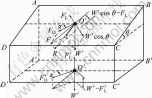
Fig. 1 Force imposed on sediment with inclined bed presented

As for sediments on horizontal bed, the critical bed shear stress can be obtained from

                         (16)

where τ′_b,cr is critical bed shear stress for sediments on horizontal bed; θ_cr is the shields number [14].

The variation of bed elevation can be derived from equation of sediment transport rate, i.e.,

                            (17)

where n is the sediments voidage.

2.3 σ-grid

With scouring development, sediments on the bed close to piers may be moved away gradually, and the plane bed may not be maintained. This will result in inclined bed surface, and gradually form the scour hole around the bridge pier. On application of CFD to the calculation of flow field around the pier, computational grids should be re-meshed since the computational domain is changed concerning the bed scouring. Since the scour hole may be of complex configuration, re-meshing of the computational domain with high quality may present a challenge.

There are three re-meshing strategies which are widely used to fit the complex terrain after scouring, i.e., Z-level grid; Shaved grid and σ-grid, as shown in Fig. 2. One can see that the represented river bed will be zigzag if the Z-level grid system is applied, which does not capture the real bed configuration. The Shaved grid may fit the complex terrain well. However, it may be very difficult to refine the mesh close to the river bed surface. In this work, the σ-grid is employed to fit the scoured bed terrain, which can provide good representation of bed terrain, while grids quality is still maintained.

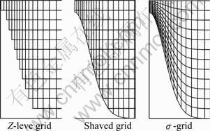
Fig. 2 Comparison between three grids systems

The relationship between the coordinate in σ-grid system and that in Cartesian coordinate system can be established by

                                 (18)

where ζ and H are the water elevation and river bed elevation from the reference plane, respectively. On the bed surface, z＝-H and σ＝-1; on free water surface,   z＝ζ and σ＝0.

3 Case study

In order to validate the effectiveness of the present method, numerical simulations of flow field as well as river bed scouring around a cylindrical pier are carried out based on available reference reports. The simulation parameters are almost the same as those reported by MELVILLE [15], except for the domain length, boundary conditions imposed on the side surface because of the available computer resource. The test was conducted in water flume of 19 m long, 45.6 cm wide, with water depth of 15 cm. A cylinder with diameter of D=5.08 cm was simulated as a scaled bridge pier fixed on the river bed. The bed sediments involved were sand with relatively uniform size, and the median grain size was 0.385 mm. The approach mean flow velocity was 0.25 m/s. Water was discharged at the rate of 0.017 12 m³/s with a bed slope of 1/10 000. Figure 3 shows the schematic plot of the test arrangement.

3.1 Computational domain and numerical methods

The computational domain, as shown in Fig. 4, is 0.15 m deep and 45.6 cm wide, with the inlet boundary locates at a distance of 7D upstream of the pier and the outlet boundary locates at a distance of 10D downstream the pier. With the development of local scour hole, the bed terrain will be modified, which means that the bottom boundary will move with the scour time. Hence, the computational domain will change because of the moving bottom boundary.

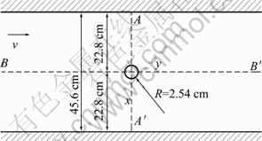
Fig. 3 Schematic plot of test arrangement

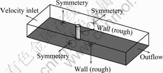
Fig. 4 Computational domain and boundary conditions

The computational domain is discretized with hexahedral blocks. In order to reflect the gradient of flow variables in the computational domain, non-uniform meshing strategy is applied, with fine grids covering the regions of interest, such as the flow field near the river bed and the pier, while grids are gradually stretched when moving away from solid surfaces. There are totally 87 948 blocks in computation domain, as shown in   Fig. 5.

For numerical simulations, boundary condition should be specified at particular location, such as inlet, outlet, solid surfaces and free surface. Their reasonable definitions are very important as to satisfy the real physics. As shown in Fig. 6, no-slip condition is applied on solid surfaces, including the bed and pier surfaces, where the former is treated as smooth surface, and the latter is treated as rough one, with the roughness height on the riverbed of 2.5d₅₀. Because of the limited computer resource, a symmetric condition is imposed on the two side surfaces and top surface. Such kind of treatment may introduce error in flow simulation, since the real top boundary is actually a free surface.

The outlet boundary uses the fully developed turbulent flow. For inlet, the velocity profile and turbulence are not available from tests. In this work, an independent three-dimensional simulation of flow is carried out in the same empty computational domain with the standard k-ε turbulent model and other simulation parameters, even the same grids system. After sufficiently long time simulation, a relatively stable speed and turbulent profile will be established, which will be transferred to the inlet boundary of simulation with the pier included. This seems to be a reasonable boundary condition since it may be consistent with the grids system, the imposed boundary condition and the employed turbulent model. For turbulence, the turbulence kinetic energy and turbulent dissipation rate are determined by k=1.5×(0.06U)² and  (0.09h), respectively.

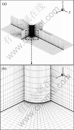
Fig. 5 Mesh arrangement around pier: (a) Grids system;      (b) Grids close to pier

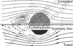
Fig. 6 Computed streamlines in comparison with test results

The experiments reported by MELVILLE [15] include two parts, i.e., the fixed-bed experiment and the live-bed experiment. In the former case, scouring will not be considered, which helps to present the flow field characteristics before scour initiation, while the live-bed experiment will simulate the evolution of the scour hole considering sediment transport. In order to validate the numerical method step by step, the results in the same conditions are also presented, and the comparison to the test results is made.

For the fixed-bed simulation, the governing equations are discretized on collocated grid system by means of the finite volume method. A second order upwind scheme is employed for the convective term, while the viscosity term uses a second order central difference scheme. The SIMPLEC algorithm is employed to solve the discretized equations. Only steady state simulation is carried out.

Except for the instantaneously changed bottom boundary as the result of bed scouring, the live-bed simulation uses the same modeling parameters. For   the unsteady simulation, the time step size is 0.01 s and total simulation ends after 180 000 time steps calculations.

3.2 Simulation results

3.2.1 Fixed-bed simulation

The velocity and bed shear stress distribution can be obtained from CFD calculation. Figure 6 shows the streamlines on the plane 2 mm on the bed surface. In order to make a direct comparison between the test and present results, the computed results (top half) is plotted against the test results (bottom half) in Fig.6. It can be seen that the presented flow features match well with the test results, such as the reversed zone downstream of the pier.

Figure 7 shows both the simulated (a) and measured (b) velocities projected to the B-B′ plane (see Fig. 3). The simulated results agree well with the test results. Also, one can see that when flow approaches the pier, it gradually changes direction and becomes downflow. The downflow is one of the principle features of flow around the pier. As one can see in the following live-bed simulation, the downflow impinges on the bed act like a vertical jet eroding a groove immediately adjacent to the front of the pier, which gradually forms the local scour hole.

Figure 8 shows a snapshot of shear stress contours on bed surface around the pier. There is a large region behind the pier showing low shear stress value, even the leading area of the pier also gets low stress value. The high stress regions are located at both sides of the pier facing the flow, indicating significant velocity gradient among the regions, especially close to the pier, where the scour may first initiate when sediments satisfy the scouring conditions.

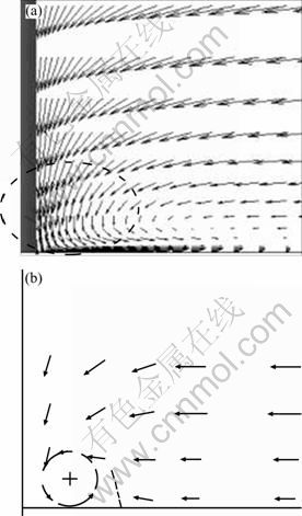
Fig. 7 Velocity distribution at plane B-B′: (a) Numerical results; (b) Experimental results

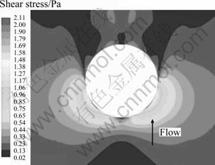
Fig. 8 Shear stress contours on bed surface

3.2.2 Live-bed simulation

In this work, the mean approach flow velocity is 0.25 m/s, with sediments average diameter of 0.385 mm, which is significantly larger than the value of U²/(g·360)=0.017 7 mm. Hence, bed load will be the major transport form.

Because of the limitation of the computational resource, the evolution of scour hole is simulated for only 30 min after scour initiated. Figures 9, 10 and 11 show the grid system at plane A-A′ at the scouring time of 10 min, 20 min and 30 min, respectively. It can be seen that the σ-grid shows good ability to follow the scouring terrain with high resolution.

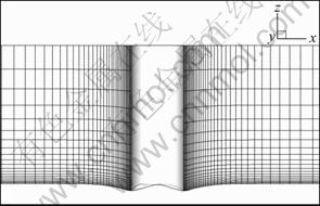
Fig. 9 Grids in vicinity of pier at 10 min

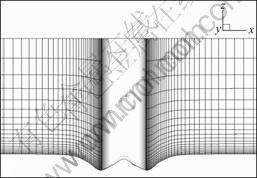
Fig. 10 Grids in vicinity of pier at 20 min

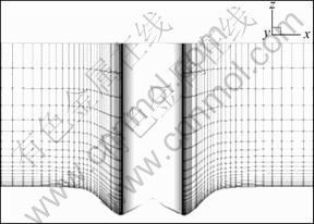
Fig. 11 Grids in vicinity of pier at 30 min

Figure 12 compares the computed scour hole shape with the experimental result at the scouring time of 30 min. The maximum scour depth observed in experiment is 4 cm and locates at the area close to the pier nose; while the maximum scour depth from the present study is 4.1 cm, and locates at pier sides. Hence, the presented maximum scour depth agrees well with the test. However, the scour hole shape and location between the numerical simulation and the test are quite different. One can see that the predicted scouring at the area immediately adjacent to the pier nose is not so intensive as that indicated in the test, i.e., there is a double-sided sharp slope immediately close to pier nose in numerical results, which may collapse in local avalanches of sediment into the erosion zone under the action of turbulent flow in the test. Such kind of collapse may change the shape of scour hole and certainly result in different flow patterns around the pier. However, such kind of slope collapse may be quite different to model, and thus is not considered in the present study.

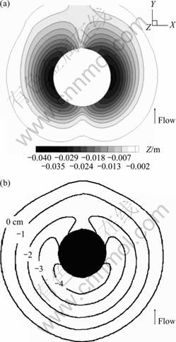
Fig. 12 Scour hole shape (t=30 min): (a) Numerical scour contours; (b) Experimental results

Figure 13 shows comparisons of velocity contours between the experiments and the numerical simulations on B-B plane at scouring time of 30 min. Both the simulated and test velocities are normalized by the mean approach flow velocity (0.25 m/s). One can see that the simulated velocity distribution agrees well with the test results, although there is slight difference in velocity gradient normal to the slope. The numerical simulation also predicts the downflow in the area close to the pier nose.

In order to present the development and profile of the scour hole, three azimuthal planes are arranged, as shown in Fig. 14. On each plane, the scour hole shape is characterized by the bed altitude stretched from the pier surface to a radial distance of 3.71 cm. Eighteen monitor points with equal interval are set to present more detailed information of scour hole shape.

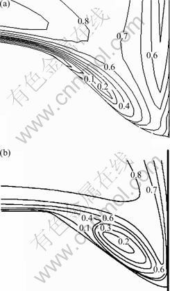
Fig. 13 Velocity (m/s) contours (t=30 min): (a) Numerical results; (b) Experimental results

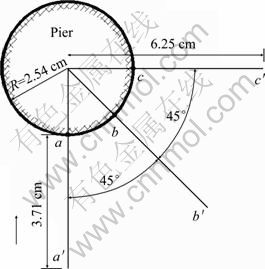
Fig. 14 Azimuthal planes arrangement

Figures 15(a), (b) and (c) show the simulated bed slope evolutions on the plane parallel to the flow direction, normal to the flow direction and between them, respectively (see Fig. 14). The horizontal axis x is the radial distance from the pier surface, while the vertical axis indicates the scour hole depth, in which zero at the vertical axis corresponds to the river bed altitude before scouring. It is shown in Fig. 15 that the maximum depth (4.1 cm) occurs at 30 min at point c. This also indicates that remarkable bed scouring occurs at the region roughly one radium away from the pier surface, with the maximum scour depth close to the pier surface line on the place normal to the flow direction.

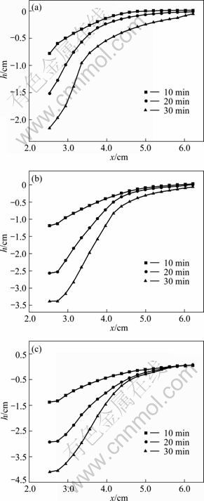
Fig. 15 Scour hole profiles evolution on three azimuthal planes: (a) a-a′ plane; (b) b-b′ plane; (c) c-c′ plane

Figure 16 shows a three-dimensional picture indicating the scour hole around bridge pier after 30 min scouring. One can see that the simulated scouring develops mainly beside the pier.

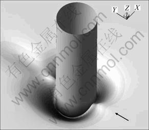
Fig. 16 Scour hole topography after 30 min scouring

4 Conclusions

1) The CFD methods, with the powerful flow visualization, show the ability of flow representation during local scouring. This helps to recognize scour mechanism and development with scour time.

2) It appears that the present three-dimensional RANS equations combined with the standard k-ε turbulence model can predict the complicate flow field around bridge piers. The accurate capture of shear stress value on the river bed is a crucial step for bed scouring.

3) The maximum scour hole depth, which is the most important parameter in scour prediction, is in good agreement with the test results. From engineering point of view, the present numerical method can be used to predict local scour hole and helps to carry out scour design of bridge piers.

4) The location of the maximum scour hole depth and the configuration predicted by present method are different from those reported by tests. This may attribute to the fact that slope collapse to the erosion zone in the test is not recognized by numerical method. Such kind of collapse may change the intermediate shape of scour hole and result in different flow patterns around the pier, and finally fail to reproduce the correct scour hole shape. Such kind of influence should be modeled in the future studies.

References

[1] CHANG H H. Fluvial processes in river engineering [M]. New York: John Wiley and Sons, 1988: 20-35.

[2] MELVILLE B W, COLEMAN S E. Bridge scour [M]. Colorado, Water Resources Publication, LLC, 2000: 8-14.

[3] National Transportation Safety Board (NTSB). Collapse of New York Thruway (I-90) Bridge over the Schoharie Creek, near Amsterdam, New York, April 5, 1987, Highway Accident Report: NTSB/HAR-88/02 [R]. Washington D C, NTSB, 1988.

[4] BARBHUIYA A K, DEY S. Measurements of turbulent flow field at a vertical semicircular cylinder attached to the sidewall of a rectangular channel [J]. Flow Meas Instrum, 2004, 15: 87-96.

[5] KANDASAMY J K, MELVILLE B W. Maximum local scour depth at bridge piers and abutments [J]. J Hydraul Res, 1998, 36: 183-197.

[6] KOTHYARI U C, GARDE R J, RANGA RAJU K G. Temporal variation of scour around cylindrical bridge piers [J]. J Hyd Engrg ASCE, 1992, 118(8): 1091-1106.

[7] PENG Jing, NOBUYUKI T, YOSHIHISA K. Three dimensional numerical simulation for sour around the head of spur dikes [J]. Journal of Sediment Research, 2002, 1: 25-29.

[8] YE Zhen-guo, WEN De-sun. Hydraulics [M]. Beijing: China Communications Press, 2001: 298-304. (in Chinese)

[9] CUI Zhan-feng, ZHANG Xiao-feng, FENG Xiao-xiang. Numerical simulation on scour around spur-dike by 3D turbulent model [J]. Journal of Hydrodinamics(A), 2008, 23(1): 33-41. (in Chinese)

[10] FEREIGER J, PERIC M. Computational method for fluid dynamics [M]. Berlin: Springer, 2002: 292-302.

[11] ABDEL-FATTAH S, AMIN A, VAN RIJN L C. Sand transport in Nile River, Egypt [J]. J Hydraul Eng, 2004, 130(6): 488-450.

[12] WANG Qiang. The finite element ocean model and its aspect of vertical discretization [D]. Bremen: University of Brement, 2007.

[13] WEI Yan-ji, YE Yin-can. 3D numerical modeling of flow and scour around short cylinder [J]. Journal of Hydrodynamics A, 2008, 23(6): 655-661. (in Chinese)

[14] QIAN Ning, WAN Zhao-hui. Sediment transport mechanics [M]. Beijing: Science Press, 2003: 233-237. (in Chinese)

[15] MELVILLE B W. Local scour at bridge sites [R]. Auckland: The University of Auckland, 1975.

(Edited by YANG Bing)

Foundation item: Project(50978095) supported by the National Natural Science Foundation of China; Project(IRT0917) supported by the Program for Changjiang Scholars and Innovative Research Team in Chinese University; Project supported by China Scholarship Council

Received date: 2011-04-11; Accepted date: 2011-09-21

Corresponding author: ZHU Zhi-wen, Professor; Tel: +86-731-88821424; E-mail: zwzhu@hnu.edu.cn