A method combining refined composite multiscale fuzzy entropy with PSO-SVM for roller bearing fault diagnosis
来源期刊:中南大学学报(英文版)2019年第9期
论文作者:谢伟达 许凡
文章页码:2404 - 2417
Key words:refined composite multiscale fuzzy entropy; roller bearings; support vector machine; fault diagnosis; particle swarm optimization
Abstract: Combining refined composite multiscale fuzzy entropy (RCMFE) and support vector machine (SVM) with particle swarm optimization (PSO) for diagnosing roller bearing faults is proposed in this paper. Compared with refined composite multiscale sample entropy (RCMSE) and multiscale fuzzy entropy (MFE), the smoothness of RCMFE is superior to that of those models. The corresponding comparison of smoothness and analysis of validity through decomposition accuracy are considered in the numerical experiments by considering the white and 1/f noise signals. Then RCMFE, RCMSE and MFE are developed to affect extraction by using different roller bearing vibration signals. Then the extracted RCMFE, RCMSE and MFE eigenvectors are regarded as the input of the PSO-SVM to diagnose the roller bearing fault. Finally, the results show that the smoothness of RCMFE is superior to that of RCMSE and MFE. Meanwhile, the fault classification accuracy is higher than that of RCMSE and MFE.
Cite this article as: XU Fan, Peter W TSE. A method combining refined composite multiscale fuzzy entropy with PSO-SVM for roller bearing fault diagnosis [J]. Journal of Central South University, 2019, 26(9): 2404-2417. DOI: https://doi.org/10.1007/s11771-019-4183-7.

J. Cent. South Univ. (2019) 26: 2404-2417
DOI: https://doi.org/10.1007/s11771-019-4183-7

XU Fan(许凡), Peter W TSE(谢伟达)
Department of Systems Engineering and Engineering Management, City University of Hong Kong,Hong Kong 990777, China
 Central South University Press and Springer-Verlag GmbH Germany, part of Springer Nature 2019
Abstract: Combining refined composite multiscale fuzzy entropy (RCMFE) and support vector machine (SVM) with particle swarm optimization (PSO) for diagnosing roller bearing faults is proposed in this paper. Compared with refined composite multiscale sample entropy (RCMSE) and multiscale fuzzy entropy (MFE), the smoothness of RCMFE is superior to that of those models. The corresponding comparison of smoothness and analysis of validity through decomposition accuracy are considered in the numerical experiments by considering the white and 1/f noise signals. Then RCMFE, RCMSE and MFE are developed to affect extraction by using different roller bearing vibration signals. Then the extracted RCMFE, RCMSE and MFE eigenvectors are regarded as the input of the PSO-SVM to diagnose the roller bearing fault. Finally, the results show that the smoothness of RCMFE is superior to that of RCMSE and MFE. Meanwhile, the fault classification accuracy is higher than that of RCMSE and MFE.
Key words: refined composite multiscale fuzzy entropy; roller bearings; support vector machine; fault diagnosis; particle swarm optimization
Cite this article as: XU Fan, Peter W TSE. A method combining refined composite multiscale fuzzy entropy with PSO-SVM for roller bearing fault diagnosis [J]. Journal of Central South University, 2019, 26(9): 2404-2417. DOI: https://doi.org/10.1007/s11771-019-4183-7.
1 Introduction
As one of the key components of rotating machinery equipment, roller bearings and their operating status affect the safety of the whole mechanical system directly. Effective monitoring and fault diagnosis of rolling bearings are needed to ensure safe manipulation of the system [1-4]. These are implemented in two steps: fault feature extraction and fault diagnosis.For roller bearings, vibration signal analysis is one of the most common and useful ways of fault extraction. Because the vibration signals have unstable and nonlinear characteristics, fault diagnosis has been challenging in recent years. Since the characteristics of roller bearing vibration signals are non-linear and show non-flat stability, many feature extraction methods, such as spectral kurtosis [5, 6], sparsity-guided empirical wavelet transform [7], approximate entropy (AE), sample entropy (SE), and fuzzy entropy (FE) have been widely and successfully used in physiological signal processing and mechanical fault diagnosis. Entropy has become one of the new ways of non-linear time series analysis. The AE method was first introduced by PINCUS et al [8] and YAN et al [9] who diffusely utilized it in fault diagnosis. However, the AE value is lower than the expected value, and the correlation is not good, especially when the data length is short. In order to overcome this shortcoming, a method known as SE is proposed and employed in successful mechanical system fault diagnosis [10, 11]. But the SE model adopts the similarity distance from any two coarse-grained time series that exceed a fixed value. However, if a fixed value is used to determine the similarity of two sequences, the SE value may be unstable. Therefore, the SE values have a mutation problem. To solve this drawback, a method called fuzzy entropy (FE) [12, 13] has introduced the exponential function to judge the resemblance between two any-time series. Compared with SE, a pre-fixed value, the fuzzy exponential function, can remove the influence of the baseline when determining sequence similarity. Hence the smoothness of the FE is overall superior to that of SE. It should be noticed that SE and FE only reflect the irregularity and the complexity of the signal on a single scale. It is difficult for a single value, such as SE and FE, to reflect all the characteristics of the signal and also difficult to construct a vector of features to complete fault diagnosis. Therefore, a method called multiscale entropy (ME) is presented to judge time-series complexity and irregularity [14, 15], in which the degree of irregularity and self-similarity of a time sequence can be shown and observed in various scales. For example, roller bearing vibration signals under outer race and inner race fault conditions can be classified by using the characteristics of the spectrum when it is working at an unusual frequency. When the roller bearing fails, the frequency of the vibration signal is different, and the corresponding complexity is also different. Therefore, ME can be considered as the characteristic index of fault diagnosis [16]. Moreover, multi-scale sample entropy (MSE) and multi-scale fuzzy entropy (MFE) have been successfully and widely used in fault diagnosis. [17-19].
However, because the SE model adopts the similarity distance from any two coarse-grained time sequences, it exceeds a regular value. Hence MSE has the following problems: undefined and no template vectors matched to other vectors. These drawbacks will affect the reliability of the MSE algorithm negatively. In order to overcome this shortcoming, WU et al [20] presented a model called refined composite multiscale sample entropy (RCMSE). The main purpose of RCMSE is to promote the precision of entropy estimation and depress the possibility of existing undefined MSE.
As mentioned above, in order to overcome the mentioned problems in SE and MSE (including the problem of unstable mutation) and also to take full advantage of FE and RCMSE, because the smoothness of the FE is overall superior to that of SE and RCMSE, FE is used to promote the precision of entropy estimation and depress the possibility of existing undefined MSE. Therefore, refined composite multiscale fuzzy entropy (RCMFE), which is combined with RCMFE and FE, is proposed in this study.
To verify that the stability and the feature extraction performance of RCMFE are better than those of MSE, RCMSE and MFE, two different signals, white and 1/f noise signals, are used in this paper. Then validity and accuracy are considered in the numerical experiments to verify that the smoothness of the RCMFE algorithm is better than that of MSE, RCMSE and MFE. After comparison and analysis by using the white and 1/f noise signals, the RCMFE algorithm is also utilized to extract useful features under various conditions. Hence the RCMFE is used to decompose the original vibration for feature extraction.
For fault diagnosis, support vector machine (SVM) is a machine learning method based on the statistical learning theory, which solves the small- sample, non-linear and high-dimensional, over- fitting and poor convergence shortcomings [21-24]. It has been widely used in roller bearing fault diagnosis [25-28]. Hence, the SVM model is regarded as the classifier to affect the fault diagnosis in this paper.
However, it is problematic to select the available parameters, so the penalty parameter C and the kernel function parameter g are included for the radial basis function (RBF) kernel in SVM, which affects the final classification accuracy. Particle swarm optimization (PSO), proposed by EBERHART [27], which is inspired by the social behavior of bird flocking and fish schooling is a global optimization technique. PSO algorithm has the following advantages: fast convergence speed; fewer adjustment parameters; better optimization effects [29, 30]. Therefore, the penalty parameter C and the kernel function parameter g, are considered as the particles in PSO to obtain the best parameters in SVM. Moreover, the identification accuracy is regarded as the fitness object function in PSO.
As mentioned above, combining RCMFE with PSO-SVM, as a fault classification method (RCMFE-PSO-SVM) for roller bearing fault diagnosis is proposed, with experimental validation in this study. The structure of the paper is organized as follows. In Section 2, a review of MFE, RCMSE, RCMFE and PSO-SVM models is presented. The comparison of MSE, MFE, RCMSE and RCMFE, including validity and accuracy, is given in Section 3. Section 4 describes the process of the method presented and parameter selection for different models. The experimental data sources and experiment validation are shown in Section 5. Lastly, the conclusions are given in Section 6.
2 Theoretical framework of MFE, RCMFE and PSO-SVM models
2.1 Basic principle of fuzzy entropy
FE is an improved method of SE which measures the regularity of the original signal. It uses the exponential function to evaluate two sequences by similar r between m points and remaining r of each other at the next point. For a time sequence with N data points, the procedure of SE calculation is as follows:
1) For the m-length vectors Xm(i)

 (1)
(1)
where m is the embedding dimension parameter, N is the length of the sample and Xm(i) contains m continuous values. Start with the ith data point and produce by eliminating a baseline:
 , 1≤j≤m (2)
2) For each Xm(i), the similarity degree between the Xm(i) and its adjacent vector Xm(j) is calculated by  as:
as:
 (3)
(3)
where denotes the maximum absolute difference between Xm(i) and Xm(j).
3) For each Xm(i) and the preconfigured similar tolerance r, Ai is the number of vectors that satisfy  , then
  is calculated by
 (4)
(4)
4) The mean value of is
is
 (5)
(5)
where r indicates the boundary width of the exponential function.
5) Increase m to m+1, then repeat steps 1)-4) to compute the SE values to find  FE can be defined as the following equation:
 (6)
(6)
The FE can be calculated by the following equation when N is finite.

 (7)
(7)
SE determines the time sequence irregularity on a single scale. The smaller the value of FE, the higher the time sequence self-similarity that can be achieved. Conversely, the greater the FE value, the more complicated the time sequences without rules that can be achieved.
2.2 Multiscale entropy and multiscale fuzzy entropy
ME is defined as the time sequences under various scales and obtained by the coarse-grained preprocess. Moreover, ME describes the irregularity of the original signal. If the entropy value of a sequence is higher than that of another sequence in most scale entropy values, then the former one is more complex than the latter one. If a time series increases with the scale factor while the entropy value monotonically decreases, this indicates that the sequence structure is relatively simple.
The MFE calculation process is given in the following steps:
1) For a discrete-time series {Xm(i):1≤i≤N}, similar tolerance r and embedding dimension m in SE are preconfigured. A new vector time sequence called coarse-grained vector 
 is constructed in sequence.
 (8)
(8)
where the parameter τ is the scale factor. It should be noted that the coarse-grained time series is the original time series {Xm(i)} when τ=1, hence the original time sequence is decomposed into a coarse-grained vector series  the number and length of coarse-grained time sequence
  are τ and N/τ, respectively.
2) The FE values are calculated according to a different scale factor τ. Here r in SE generally takes the standard deviation (SD) from the original time sequences. Therefore, MFE can be defined by:
 (9)
(9)
2.3 Basic principle of RCMFE
The time series length is decreased by the parameter τ. To analyze the short time series, the MFE model usually induces inaccurate FE when the scale is large. Hence WU et al [20] presented a method known as RCMSE to enhance the precision of the MSE. In the RCMSE, all the coarse-grained time sequences are computed by scale factor τ. The RCMSE value is calculated by:
 (10)
(10)
where  and
and 
 Thus the RCMSE value can be defined as:

 (11)
(11)
RCMFE is an improved method of RCMSE which measures the regularity of time series with Eqs. (2)-(3).
 (12)
(12)
2.4 PSO-SVM model
1) The basic theory of SVM is derived from statistical learning. Because the number and information of samples are limited; the purpose of SVM is to find a compromise between the learning ability and model complexity. The detailed calculation of SVM is given in Ref. [28] and shown as follows.
For a given training dataset 
 where xt denotes the input vector, xlabel is the data label, and k indicates the number of categories. Binary classifiers construct the multi-class classifiers, which are known as one-against-one SVM. In the SVM training process, the binary classification problem can be defined by the following equation:
 (13)
(13)

 (14)
(14)
where  denotes a slack variable; C indicates a penalty constant; b and
  are paranoid items and the high dimensional transformation of xt. The Lagrange multiplier operation is used to map the xt into high dimensional through the incorporating kernels. The aforementioned question is transformed into a quadratic optimization problem as follows:
 (15)
(15)
where K(x, xt) denotes the kernel function;  is the Lagrange multiplier. The SVM applied the following strategy to make a decision for each sample. If sample x appertains to the ith class by using f ij(x), then the vote for the ith class is added by one. After the total classifiers (k*(k-1)/2) have finished the identification task with all samples, x appertains to the class which has the maximum number of votes.
Because the RBF has good properties and universal usage, we use the RBF. The RBF definition is given as follows:
 (16)
(16)
2) PSO algorithm. The swarm has m particles. Two parameters, velocity 
 and the current position
 are used to depict each particle. Here is the particle dimension number. The best position Pbestd(t) moves according to a search space with n dimensions.
The PSO aims to search the best position by all particles using the updated position in each iteration.
The global position Gbestd(t) denotes the best position at the current generation. Here t represents the current iteration. The velocity and position of each particle are generated and updated by:

 (17)
(17)
 (18)
(18)
In the above formula, the velocity Vi and position Xi are restricted to the [-Vmin, Vmax] and [-Xmin, Xmax]. Here Vmax and Xmax are the predefined maximum values for the velocity Vi and position Xi. r1 and r2 are ranged in [0,1] randomly. The parameters c1 and c2 are constant values. The related and detailed procedure of SVM parameter optimization by using the PSO algorithm is given as follows:
1) Initialization. For each particle, initialize the position and velocity randomly. The total number of the particles (n) is preset before SVM training, the maximum iteration tmax, and weight (w) are fixed at the same time. Execute the training process according to the following steps 2)-6).
2) Set iteration variable. Increase t in each iteration, t=t+1.
3) Fitness evaluation. Assess the quality of every particle before finding the optimal values in SVM including the parameters C and g. The fitness function on the bias of identification accuracy of an SVM classifier is selected as the optimization goal. The definition of fitness function is given as:
 (19)
(19)
where sumerror and sumright represent the right and error identification number, respectively.
4) Stop condition checking. When the value of the fitness function is smaller than the stopping criteria, which are predefined by the error accuracy ε. If the iteration number exceeds the maximum iterations, go to step 6). Otherwise, go to step 5).
5) Update. For each particle, the velocity and position are updated by using Eqs. (17)-(19). The next step is to go to step 2).
6) End condition. In this step, the parameters C and g are selected.
3 Simulation analysis of MSE, RCMSE, MFE and RCMFE
In order to compare the effect of the MSE, RCMSE, MFE and RCMFE, two kinds of signals, white and 1/f noise signals, were used to compare. Validity and accuracy were utilized in the numerical experiments. The MSE, RCMSE, MFE and RCMFE values under different scales from 1 to 20 were calculated in this section, the parameter- embedded dimension m and similar tolerance r in MSE, MFE, RCMSE and RCMFE were selected as 2 and 0.15 SD, respectively, where SD was the standard deviation from the original signal.
3.1 Comparison of validity
The possibility of undefined entropy was used to compare the white and 1/f noise signals for 200 samples by using MSE, RCMSE, MFE and RCMFE models. The length of each sample was 1000. The corresponding probabilities are given in Table 1. In Table 1, the possibility of undefined entropy increased as the scale factor increased, while the lengths of the coarse-grained time sequences decreased.
As shown in Table 1, the possibility of the undefined entropy is zero when it is applied to analyze white noise in MSE. In contrast, the possibility of undefined entropy is 0.01 when τ=4 with 200 1/f noise samples. The entropy is undefined when Bm(r) or Bm+1(r) is zero in MSE. However, the MSE, RCMSE, MFE and RCMFE are used to compute the entropy values well. Hence the MFE/RCMSE/RCMFE models are superior to the MSE model.
3.2 Comparison of accuracy
The accuracy of the MSE, RCMSE, MFE and RCMFE models is verified in this section. Two hundred noise samples with 1000 data points, including white and 1/f noise, were considered in each simulation. The results of MSE, RCMSE, MFE and RCMFE entropies are given in Figure 1, the standard deviations (SDs) and means of entropies are also given in Figures 2 and 3. As shown in Figure 1(a), regarding white noise, the overall smoothness of RCMSE/MFE/RCMFE models is superior to that of the MSE model, because the similarity tolerance r in SE is employed to measure the similarity between two anytime series, here r is a constant which is often set as 10%-25% of the standard deviation.
Table 1 Probabilities of inducing undefined entropy for white and 1/f noise signals by using MSE, RCMSE, MFE and RCMSE
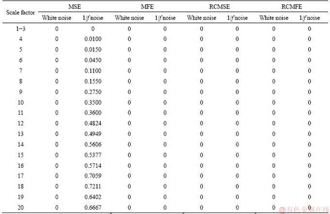

Figure 1 MSE/RCMSE/MFE/RCMFE values of white and 1/f noise signals:
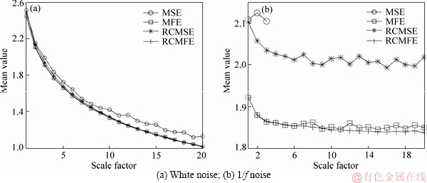
Figure 2 Mean value of MSE/RCMSE/MFE/RCMFE with white and 1/f noise signals:

Figure 3 Standard deviation value of MSE/RCMSE/MFE/RCMFE with white and 1/f noise signals:
Figures 2(a) and (b) show that the average of the entropy values by using the MSE/RCMSE/ MFE/RCMFE is nearly equal in white noise. Nevertheless, the mean value of the entropy of the MSE/RCMSE/MFE is higher than that of the RCMFE (see Figure 2(b)). Figure 3 shows that the SD of RCMFE is lower than that of the MSE/RCMSE/MFE models. These results indicate that the entropies obtained by using the RCMFE are more consistent than those obtained by using the MSE/RCMSE/MFE algorithms.
To compare the effect of data length on the MSE/RCMSE/MFE/RCMFE, the entropies of 1/f noise at a time scale of 20 ( =20) were calculated using several data lengths (N=500, 1000, 1500 and 2000). The means and standard deviations of the entropies are shown in Table 2.
The averages of the entropies using these four models were close to equivalent when the data length was long, such as N=2000, but when the length of the original time series was short, they were different. Consider the differentiation between the entropy of 1/f noise when N=500 and N=2000. The result from the RCMFE algorithm is the lowest among these three models. The smaller the mean and standard deviations of all samples when using RCMFE, the stronger the stability of RCMFE [20]. In other words, the RCMFE outperformed the other three models in terms of the independence of the length of data when the time series was characterized. Based on the above discussions, compared with other models, the RCMFE algorithm is the most stable and reliable model.
4 Procedures of proposed method and parameter selection
4.1 Procedures of proposed method
In this section, the detailed procedures of the proposed method are given in the following steps:
1) All the vibration signals under various conditions were decomposed by RCMSE, MFE, and RCMFE.
2) The extracted ME values at the first step were regarded as the input of RCMSE, MFE and RCMFE to diagnose the faults. But training samples were used in training the SVM with PSO. The best penalty parameter C and the kernel function parameter g in SVM were found in this step.
3) The reminder samples and testing samples were used to test the built model SVM with PSO at the second step. To demonstrate that the performance of the proposed model, RCMFE-PSO- SVM, was better than that of other combined models, such as MFE/RCMSE-PSO-SVM, the classification accuracy was used in the final step.
As mentioned above, the flowchart of the proposed fault model is shown in Figure 4.
4.2 Parameter selection for different methods
In order to effect fault diagnosis, some important parameters should be preconfigured in various models.
Table 2 Means and standard deviations of MSE/MFE/RCMSE and RCMFE of 1/f noise at a scale factor of 20

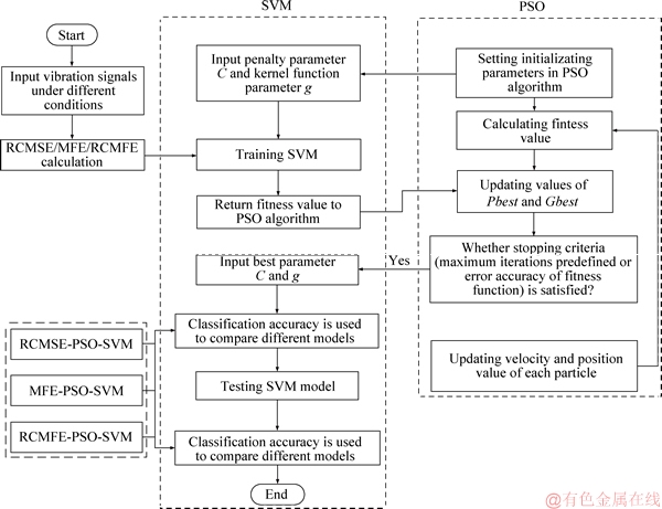
Figure 4 Flowchart of proposed method
1) SE and FE. Embedding dimension m and similarity tolerance r, these two parameters are important in SE and FE. m must meet one requirement N=10m-30m, where N is the length of data. The authors in Refs. [11-17, 32-37] suggest that m is often fixed as 2. Another parameter r is utilized to measure the gradient and range of the data. The greater the r is, the more useful the information will be lost. The smaller the r is, the more possible the salient influence will be submerged in noise.
Particularly, r is set as 0.1-0.25 SD from the original series; here SD is the standard deviation from the original data [11-17, 32-35].
2) PSO-SVM. The iteration number tmax is set as 200 in this study, the particle size n is chosen as 20. Meanwhile, the error classification accuracy ε=0.001. The velocity Vi and position Xi are ranged into [0.01, 1000] and [0.1, 100], respectively, positive constants c1 and c2 are fixed at 1.5 and 1.7, r1 and r2 are random numbers in [0, 1]. The parameter inertia weight w in Eq. (17) is 1.
3) In RCMSE, MFE and RCMFE, there is an important parameter known as the scale factor τ that should be set before calculation. The authors in Refs. [14-18] demonstrate that the greater the scale factor  , the greater the average precision. Too high a value of the scale factor will lead to greater computational complexity and produce more redundant information. Therefore, the scale factor τ is set as 20 in this paper. It should be noted that the scale factor τ is the dimension of the extracted ME feature after RCMSE, MFE and RCMFE decomposition.
5 Experimental results and analysis
5.1 Experimental data and setup
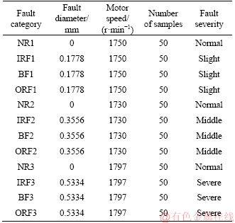
The experimental data were collected from the Case Western Reserve University Bearing Data Center of NASA in the US [31]. There are eleven kinds of roller bearing faults. For each type, 50 samples of 2048 data length are contained. The roller bearing working frequency is 12 kHz. Normal (NR), ball fault (BF), inner race fault (IRF), and outer race fault (ORF), these four types of fault under different fault diameters of 0.1778 mm (1hp), 0.3556 mm (2hp) and 0.5334 mm (3hp) are utilized in this study, where 1hp, 2hp and 3hp denote different motor speed conditions of 1750, 1730 and 1797 r/min, respectively. Hence the greater the fault diameters, the greater the degree of the fault, for example 0.1778 is slight, 0.3556 mm and 0.5334 mm are middle and severe. The related information about the experimental data is listed below in Table 3.
Table 3 Roller bearings experimental vibration data under different conditions
The original vibration signal is shown in Figure 5. It is not easy to distinguish all types of vibration signal directly at first glance. All NR signals without regularity under different conditions are similar, for example NR2 and NR3. Compared with NR, all IRF and ORF signals have obvious regularity. There is a fixed impact when roller bearings are working in IRF and ORF.
However, MFE, RCMSE and RCMFE are considered to decompose those vibration signals. The MSE, RCMSE and RCMFE values when using one sample are shown in Figure 5 when r=0.2 SD.
It can be seen from Figure 6 that all states (NR, IRF, OF, BF) are better distinguished when scale factors τ≥2, as all NR signals with random vibration characteristics cause the vibration amplitude to be small. The smaller the vibration amplitude value is, the larger the MFE, RCMSE and RCMFE are, because the ln function in Eq. (11) is a monotonically increasing function, but there is a negative operation in the final step in the MFE, RCMSE and RCMFE calculation. Therefore, all MFE, RCMSE and RCMFE signals are higher than other fault signals such as BF, IRF and ORF.
In addition, the IRF and ORF signals have fixed vibration regularity because the inner race and outer race equipment suffer a certain impact when roller bearings are spinning. This will lead to the vibration amplitude of IRF and ORF signals being greater than that of the BF signal. This can be verified from Figure 5, for example IRF3 and ORF3 signals. A descending sequence of the MFE, RCMSE and RCMFE values is NR>BF>IRF>ORF overall.
In Figure 6, when the scale factor τ increases gradually, the overall MSE value decreases. Conversely, as the scale factor τ becomes smaller (especially when τ<10), the overall trend is gradually discriminative. Therefore, it describes the situation on a smaller scale factor τ containing much information.
It can be seen from Figure 6 that the smoothness of RCMFE is superior to that of the RCMSE and MFE. Compared with MFE and RCMSE, all the NR signal lines calculated by RCMFE in Figure 6(c) closely resemble a beeline at first glance when τ>10, but there is fluctuation in Figures 6(a) and (b). Other vibration signals, such as BF, IRF and ORF signals are also the same as the NR signal. In the RCMFE, the FE of all coarse- grained time sequences is calculated. Therefore, RCMFE is the average of all the FE values under the same scale factor τ, and not of a single coarse- grained time series. Meanwhile, FE uses the exponential function to judge the resemblance among two signals, and not a fixed number of constants. Hence the smoothness of the RCMFE is superior to that of the MFE and RCMSE.
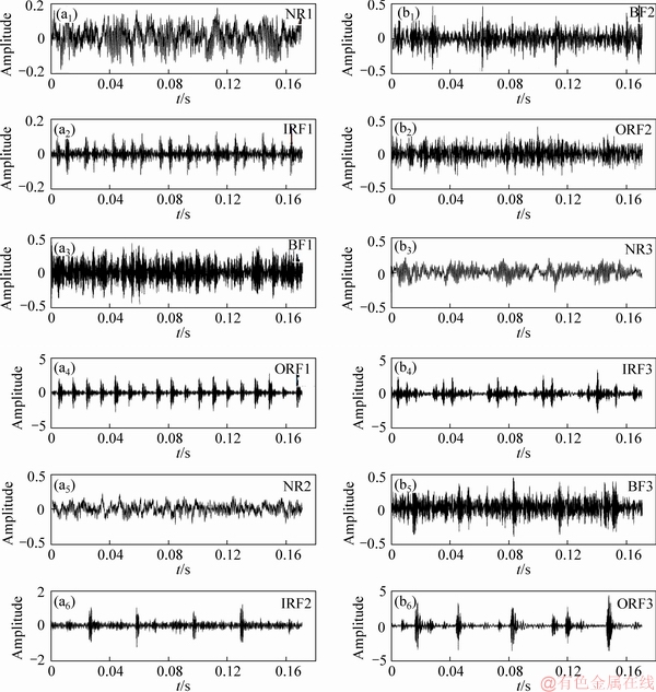
Figure 5 Original vibration signal under various faults
5.2 Fault identification
After all types of vibration signal have been decomposed by MFE, RCMSE and RCMFE, the MFE, RCMSE and RCMFE obtained are selected as the input of the SVM with PSO for fault diagnosis. The total number of each vibration signal in 50, 20 and 30 samples is chosen as the input to train SVM, and the remaining 30 and 20 samples are chosen as testing samples to test the PSO-SVM model. Therefore, the total numbers of training samples are 240 and 360, while the corresponding testing samples are 360 and 240. The best parameters C, g and the classification accuracy obtained from PSO-SVM are rendered in Tables 4 and 5. It should be mentioned that the value of scale factor τ is selected as different values, such as 2, 4, 6, 8, 10, 12, 14, 16, 18 and 20, to verify that the classification accuracy of the RCMFE is superior to that of MFE and RCMSE when using PSO-SVM. All results are listed in Table 4. In addition, we also provide some fault identification figures in Figure 7.
In Table 4, the highest classification accuracies of RCMFE, MFE, and RCMSE are 99.16%, 97.08% and 97.92%, the lowest classification accuracies are 93.05%, 88.05% and 94.16%. All the classification accuracies of RCMFE are higher than those of MFE and RCMSE (about 1%-5%), especially when compared with those of RCMSE,the values of RCMFE are about 5% higher overall.
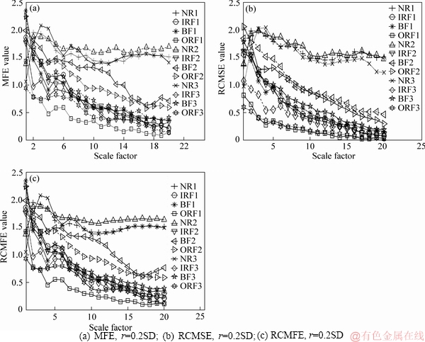
Figure 6 RCMSE, MFE, and RCMFE values for roller bearing vibration signals:
Table 4 Identification accuracy (%) when τ=4, 6, 8, 10, 12, 14, 16, 18 and 20, respectively
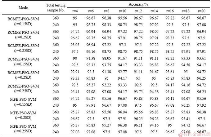
Table 5 Identification accuracy, best parameters C and g when τ=20
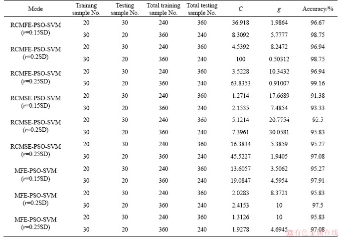

Figure 7 Results of identification accuracy between actual and predicted samples when using RCMSE, MFE, RCMFE-PSO-SVM models for roller bearings (τ=6):
It can be seen from Table 4 that the identification accuracy increases as the scale factor increases, and then maintains a steady stable condition after τ=10, specially in RCMFE, the classification accuracy values when τ=12, 14, 16, 18, 20 are ranged into 97%-98%. This is due to the fact that the RCMFE value remains stable after τ=10. This can be proven from Figure 6. Compared with RCMFE, the classification accuracy values in RCMSE and MFE are fluctuating, such as RCMSE of about 91%-97%.
In Table 5, all accuracy in RCMFE is superior to that of the RCMSE and MFE when scale factor τ=20. These results demonstrate that the identification performance is better than that of RCMSE and MFE.
6 Conclusions
In order to solve the smoothness problem, a fixed threshold is used to decide the similarity between any two sequences in SE. A method known as RCMFE is proposed. In comparison with RCMSE, RCMFE adopts the fuzzy exponential function to determine the similarity of any two sequences. To verify its superior performance in RCMFE, two types of signal, white noise, and 1/f, are considered to compare the validity and accuracy of the RCMSE, MFE and RCMFE. Then we analyze and compare from different perspectives, including the decomposition accuracy, data length and validity. Because the RCMFE uses the average of all coarse-grained sequences at the same scale, the results show that the smoothness of RCMFE is superior to that of the MFE and RCMSE at the same time. Finally, PSO-SVM is selected as the classifier to diagnose the different roller bearing faults. The experimental outcomes show that the identification accuracy of the method presented is greater than that of the other aforementioned combination methods such as RCMSE/MFE- PSO-SVM.
References
[1] HUANG Yi, WANG Bin-xing, WANG Jia-qian. Test for active control of boom vibration of a concrete pump truck [J]. Journal of Vibration and Shock, 2012, 31(2): 91-94. (in Chinese)
[2] RESTA F, RIPAMONTI F, CAZZLUANI G, FERRARI M. Independent modal control for nonlinear flexible structures: An experimental test rig [J]. Journal of Sound and Vibration, 2011, 329(8): 961-972.
[3] BAGORDO G, CAZZLUANI G, RESTA F, RIPAMONTI F.A modal disturbance estimator for vibration suppression in nonlinear flexible structures [J]. Journal of Sound and Vibration, 2011, 330(25): 6061-6069.
[4] WANG Xiang-bing, TONG Shui-guang. Nonlinear dynamical behavior analysis on rigid flexible coupling mechanical arm of hydraulic excavator [J]. Journal of Vibration and Shock, 2014, 33(1): 63-70. (in Chinese)
[5] WANG D. Some further thoughts about spectral kurtosis, spectral L2/L1 norm, spectral smoothness index and spectral Gini index for characterizing repetitive transients [J]. Mechanical Systems and Signal Processing, 2018, 108: 360-368.
[6] WANG D. Spectral L2/L1 norm: A new perspective for spectral kurtosis for characterizing non-stationary signals [J]. Mechanical Systems and Signal Processing, 2018, 104: 290-293.
[7] WANG D, ZHAO Y, CAI Y, TUSI K L, LIN J H. Sparsity guided empirical wavelet transform for fault diagnosis of rolling element bearings [J]. Mechanical Systems and Signal Processing, 2018, 101: 292-308.
[8] PINCUS S M. Approximate entropy as a measure of system complexity [J]. Proceedings of the National Academy of Sciences, 1991, 55: 2297-2301.
[9] YAN R Q, GAO R X. Approximate Entropy as a diagnostic tool for machine health monitoring [J]. Mechanical Systems and Signal Processing, 2007, 21: 824-839.
[10] RICHMAN J S, MOORMAN J R. Physiological time-series analysis using approximate entropy and sample entropy [J]. American Journal of Physiology-Heart Circulatory Physiology, 2000, 278(6): 2039-2049.
[11] ZHU K H, SONG X, XUE D X. Fault diagnosis of rolling bearings based on IMF envelope sample entropy and support vector machine [J]. Journal of Information & Computational Science, 2013, 10(16): 5189-5198.
[12] CHEN W T, ZHUANG J, YU W X, WANG Z Z. Measuring complexity using FuzzyEn, ApEn, and SampEn [J]. Med Eng Phys, 2009, 31: 61-68.
[13] XIONG G L, ZHANG L, LIU H S, ZOU H J, GUO W Z. A comparative study on ApEn, SampEn and their fuzzy counterparts in a multiscale framework for feature extraction [J]. J Zhejiang Univ Sci A, 2010, 11(4): 270-279.
[14] COSTA M, GOLDBERGER A L, PENG C K. Multiscale entropy analysis of complex physiologic time series [J]. Physical Review Letters, 2002, 89(6): 1-18.
[15] COSTA M, GOLDBERGER A L, PENG C K. Multiscale entropy analysis of biological signals [J]. Physical Review E, 2005, 71(5): 1-18.
[16] ZHENG Jin-de, CHENG Jun-sheng, YANG-Yu. A rolling bearing fault diagnosis approach based on multisclae entropy [J]. Journal of Hunan University (Natural Sciences), 2012, 39(5): 38-41. (in Chinese)
[17] ZHANG L, XIONG G L, LIU H S, ZOU H J, GUO W Z. Bearing fault diagnosis using multi-scale entropy and adaptive neuro-fuzzy inference [J]. Expert Systems with Applications, 2010, 37: 6077-6085.
[18] ZHENG J D, CHENG J S, YANG Y, LUO S R. A rolling bearing fault diagnosis method based on multi-scale fuzzy entropy and variable predictive model-based class discrimination [J]. Mechanism and Machine Theory, 2014, 78: 187-200.
[19] ZHENG J D, CHENG J S, YANG Y. A rolling bearing fault diagnosis approach based on LCD and fuzzy entropy [J]. Mechanism and Machine Theory, 2013, 70: 441-453.
[20] WU S D, WU C W, LIN S, G LEE K Y, PENG C K. Analysis of complex time series using refined composite multiscale entropy [J]. Phys Lett A, 2014, 378(20): 1369-1374.
[21] LIU Z W, CAO H R, CHEN X F, HE Z J, SHEN Z J. Multi-fault classification based on wavelet SVM with PSO algorithm to analyze vibration signals from rolling element bearings [J]. Neurocomputing, 2013, 99: 399-410.
[22] DENG W, YAO R, ZHAO H M, YANG X H, LI G Y. A novel intelligent diagnosis method using optimal LS-SVM with improved PSO algorithm [J]. Soft Computing, 2019, 23(7): 2445-2462.
[23] DENG W, ZHAO H M, ZOU L, LI G, YANG X H, WU D Q. A novel collaborative optimization algorithm in solving complex optimization problems [J]. Soft Computing, 2017, 21(15): 4387-4398.
[24] DENG W, ZHAO H M, LIU J J, YAN X L, LI Y Y, YIN L F. An improved CACO algorithm based on adaptive method and multi-variant strategies [J]. Soft Computing, 2015, 19(3): 701-713.
[25] ZHENG Jin-de, CHENG Jun-sheng, YANG-Yu. Multi-scale permutation entropy and its applications to rolling bearing fault diagnosis [J]. China Mechanical Engineering, 2013, 24: 2641-2646. (in Chinese)
[26] HAN M H, PAN J L. A fault diagnosis method combined with LMD, sample entropy and energy ratio for roller bearings [J]. Measurement, 2015, 24: 7-19.
[27] EBERHART R, KENNEDY J. A new optimizer using particle swarm theory [C]// Sixth International Symposium on Micro Machine and Human Science. Nagoya, Japan. 1995: 39-43.
[28] DENG W, ZHAO H M AND YANG X H, XIONG J X, SUN M, LI B. Study on an improved adaptive PSO algorithm for solving multi-objective gate assignment [J]. Applied Soft Computing, 2017, 59: 288-302.
[29] DENG W, CHEN R, HE B, YIN L, GUO J. A novel two-stage hybrid swarm intelligence optimization algorithm and application [J]. Soft Computing, 2012, 16: 1707-1722.
[30] GU B, SHENG V S. A robust regularization path algorithm for í-support vector classification [J]. IEEE Transactions on Neural Networks and Learning Systems, 2017, 28(5): 1241-1248.
[31] Case Western Reserve University. Bearing data center test seeded fault test data [EB/OL]. 2013. http://csegroups. case.edu/bearingdatacenter/pages/download-data-file.
[32] DENG W, ZHANG S J, ZHAO H M, YANG X H. A novel fault diagnosis method based on integrating empirical wavelet transform and fuzzy entropy for motor bearing [J]. IEEE Access, 2018, 6: 35042-35056.
[33] ZHAO H M, SUN M, WU D, YANG X H. A new feature extraction method based on EEMD and multi-scale fuzzy entropy for motor bearing [J]. Entropy, 2017, 19(1): 1-21.
[34] TANG R L, LI X, LAI J G. A novel optimal energymanagement strategy for a maritime hybrid energy system based on largescale global optimization [J]. Applied Energy, 2018, 228: 254-264.
[35] TANG R L, WU Z, LI X. Optimal operation of photovoltaic/battery/diesel/coldironing hybrid energy system for maritimeapplication [J]. Energy, 2018, 162: 697-714.
(Edited by FANG Jing-hua)
中文导读
基于精细复合多尺度模糊熵与粒子群优化支持向量机的滚动轴承故障诊断
摘要:提出了一种结合精细复合多尺度模糊熵和采用粒子群优化支持向量机滚动轴承故障诊断模型。通过使用白噪声和1/f噪声的数值仿真实验中比较平滑度和分解精度的有效性,与精细复合多尺度样本熵和多尺度模糊熵相比,精细复合多尺度模糊熵的平滑度优于这些模型。随后使用精细复合多尺度模糊熵,精细复合多尺度样本熵和多尺度模糊熵对不同状态的滚动轴承振动信号进行特征提取,将提取的特征向量作为粒子群优化的支持向量机的输入实现滚动轴承故障诊断。实验结果表明,精细复合多尺度模糊熵的平滑度优于精细复合多尺度样本熵和多尺度模糊熵,同时,故障分类精度高于精细复合多尺度样本熵和多尺度模糊熵。
关键词:精细复合多尺度模糊熵;滚子轴承;支持向量机;故障诊断;粒子群优化算法
Foundation item: Projects(CityU 11201315, T32-101/15-R) supported by the Research Grants Council of the Hong Kong Special Administrative Region, China
Received date: 2018-01-05; Accepted date: 2018-10-22
Corresponding author: Peter W TSE, Associate Professor, PhD; Tel: +852-544110285; E-mail: Peter.W.Tse@cityu.edu.hk; ORCID: 0000-0002-6796-7617

