J. Cent. South Univ. Technol. (2008) 15(s1): 181-186
DOI: 10.1007/s11771-008-342-y

Numerical prediction of inner turbulent flow in conical diffuser by using a new five-point scheme and DLR k-ε turbulence model
JIANG Guang-biao(蒋光彪)1, 2, HE Yong-sen(何永森)1, 2, SHU Shi(舒 适)1, 2, XIAO Yin-xiong(肖映雄)1, 2
(1. College of Mathematics and Computational Science, Xiangtan University, Xiangtan 411105, China;
2. Hunan Key Laboratory for Computation and Simulation in Science and Engineering,
Xiangtan University, Xiangtan 411105, China)
Abstract: The internal turbulent flow in conical diffuser is a very complicated adverse pressure gradient flow. DLR k-ε turbulence model was adopted to study it. The every terms of the Laplace operator in DLR k-ε turbulence model and pressure Poisson equation were discretized by upwind difference scheme. A new full implicit difference scheme of 5-point was constructed by using finite volume method and finite difference method.A large sparse matrix with five diagonals was formed and was stored by three arrays of one dimension in a compressed mode. General iterative methods do not work wel1 with large sparse matrix. With algebraic multigrid method(AMG), linear algebraic system of equations was solved and the precision was set at 10-6. The computation results were compared with the experimental results. The results show that the computation results have a good agreement with the experiment data. The precision of computational results and numerical simulation efficiency are greatly improved.
Key words: conical diffuser; turbulent flow; DLR k-ε turbulence model; 5-point scheme; algebraic multigrid method(AMG)
1 Introduction
A conical diffuser(Fig.1) has been widely used in engineering. The internal turbulent flow is a very complicated adverse pressure gradient flow. In Ref.[1], the low Reynolds number(DLR) k-ε turbulence model and its BFC method (boundary fit curvilinear coordinate transformation method)[2-3] were used to make the prediction of turbulent flows in a conical diffuser, the validated results were gotten. But the difference equations were constructed by the upwind difference scheme of the 3rd precision and center difference scheme, and then the equivalent equations in the computational plane were discretized by a node stencil of 13-point, large sparse matrices with 13 diagonals were formed. Because the node stencil was large and many nodes were used, the CPU time was much. In this paper, numerical prediction of inner turbulent flow in conical diffuser based on DLR k-ε turbulence model is studied and a new five-point scheme is given. By use of the combination of the finite difference method and finite volume method, the non-linear convective terms and viscosity terms were discretized by upwind difference scheme, the equivalent equations in the computational plane were discretized by a node stencil of 5-point. Large sparse matrices with 5 diagonals were formed. The sparse matrices were stored by a compressed format of three one-dimensional arrays. The difference equations were solved by algebraic multigrid method (AMG). Numerical experiments show that, with the combination of the DLR k-ε turbulence model and the algebraic multigrid method, a new algorithm for numerical prediction of inner turbulent flow was developed; by use of the improved scheme and AMG method, the efficiency and precision of numerical prediction are greatly improved.
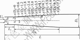
Fig.1 Model flow field in conical diffuser
2 Governing equations
By use of the elliptical differential equations[4], the body-fitted grid which is orthogonal to the boundary and clustering near wall boundary is generated. The typical generated grid of unequal intervals is shown in Fig.2. In this paper, all variables are non-dimensionalized. The dimensionless forms of the governing equations[3] in cylindrical coordinate system can be written as follows:
 (1)
(1)

 (2)
(2)


 (3)
(3)

 (4)
(4)

 (5)
(5)

 (6)
(6)


where x and r are the axial and radial coordinates;  is mean pressure; u0 is inflow velocity;
  and
and  are mean velocity components in x and r directions; k is turbulent kinetic energy;
  is turbulent dissipation rate; vt is eddy viscosity; Re is Reynolds number, Re=U0D0/v;
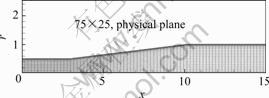
Fig.2 Typical grid of unequal intervals
Rt is turbulence Reynolds number,  ; ur is y+ is dimensionless distance from the wall,
  ; friction velocity;
  =[26, 4.1, 6.5, 6.0], are constant coefficients; [CD, C1, C2, σ1, σ2]=[0.09, 1.44, 1.92, 1.0, 1.3], are model constants.
3 Numerical method
The discretization techniques used in the present work were the finite difference method and finite volume method. The new type of discretization scheme was motivated by the authors’ experience.
3.1 Discretization of Laplace equation
The equivalent equations of Laplace equation in cylindrical coordinate system can be written as follows:

 (7)
(7)
In the following, based on upwind difference idea, Eqn.(7) is discretized by finite volume method, a new 5- point difference scheme is constructed. Every term in the Laplace equation is discretized as follows.
1) For second order derivative,


2) For one order derivative,


3) For second order mixed derivative,


The above discretized terms of all kinds of deriva- tives are put together, a new difference scheme with 5- point for Laplace equation is constructed.
3.2 Discretization of pressure Poisson equation
In this work, the pressure correction algorithm is adopted, namely based on momentum equation, the relational expression of velocity and pressure is constructed, the continuity equation is substituted into the relational expression, the pressure Poisson equation is formed after simplifying the expression. According to the body fitted coordinate transformation, the pressure Poisson equation in computational plane can be gotten and written as follows:


 (8)
(8)
where,


Similar to Laplace equation, a new 5-point difference scheme is constructed as follows:


 (9)
(9)
The above formula can be simplified as
 (10)
(10)
The meanings of subscripts are shown in Fig.3. The coefficients of the discretised equation are shown as follows:


 ;
;
 ;
;

 ;
;
 ;
;
 .
.
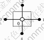
Fig.3 Node stencil of five-point difference scheme
The coefficient matrix of difference Eqn.(9) is large sparse matrix and it is of the diagonal dominance. According to the linear algebraic theory, the iterations are convergent.
3.3 Discretization of DLR k-ε turbulence model
The colocated body-fitted grids system was adopted in this work, all flow parameters were set in the same grid point. Firstly, according to the body fitted coordinate transformation, the model equations in physical plane can be transformed into the equivalent equations in computational plane, and then the equivalent equations of DLR k-ε turbulence model equations are discretized in computational plane. In order to obtain not only the accurate but also stable and convergent numerical results for improving the computational efficiency, the convective terms are discretized by upwind difference scheme of one order precision; the viscosity terms are discretized according to the discrete method of Laplace equation; as to the time term, the EULER backward scheme was adopted in the present work. For example, the  momentum equation of x direction can be discretized as follows (for convenience, the time average symbol “-” is omitted):


 (11)
(11)
The above formula can be simplified as
 (12)
(12)
where


 ;
;

 ;
;

 ;
;

 ;
;

 ;
;

where,  ,
,  ;
;  ,
,  ,
,  ,
,  ,
,  ,
,  ,
,  and
and  are the metric coefficients of transformation;
  and
and  are inverse transformation velocity vectors in
  and
and  directions respectively. In regard to other equations such as , k, ε, the discrete methods are the same, for brevity, the contents are omitted.
According to the above discrete process, the coefficient matrices of the difference equations for , , k, ε can be written as follows:
 (13)
(13)
Matrix B is a five-diagonal large spare matrix; B11, B22 and B33 are the tridiagonal submatrices; B12 and B21 are diagonal submatrices; IL and JL are the numbers of grid points in x direction and r direction, respectively.
3.4 Solution of DLR k-ε turbulence model
The DLR k-ε turbulence model has six flow parameters and six equations, so it is a closure model. The algebraic multigrid method is a popular fast algorithm which is used to solve the discrete system of differential equations. In this work, the DLR k-ε turbulence model and the algebraic multigrid method are integrated and the discrete algebraic system were solved by algebraic multigrid method[5-6]. The number of the outer iterations is controlled by the error of time level n+1 and time level n of solution. Convergence criterion is set as follows:
 (14)
(14)
4 Results and discussion
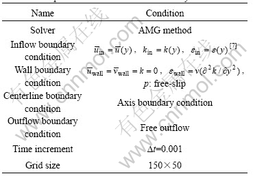
The computational example is the turbulent flow field in an axi-symmetric conical diffuser having a total divergence angle of 8? and an ratio of 4?1 with inflow Reynolds number of 2.93×10⁵ and 1.16×10⁵. The computational conditions and boundary conditions are listed in Table 1. In the present work the AMG method was chosen. By use of the scheme of new 5-point scheme and the old 13-point scheme that is often used in ever calculations, the numerical experiments are made. The computational results of and k are shown. The computational results are compared with each other and also with the experimental data by OKWOUBI and SINGH. The hardware environment of numerical experiment is: hp dx2038M (intel(R)) Pentium(R) 4 CPU, 3.06 GHz, 992 MB EMS memory; the software environment of numerical experiment is: Compaq Visual Fortran Professional Edition6.6.0.
Table 1 Computational conditions and boundary conditions
4.1 Comparison of computational efficiency
The comparison of computational efficiency between the scheme of new 5-point scheme in the present work (new scheme) and the old 13-point scheme (old scheme) that is often used in ever calculations are listed in Table 2 (Re=2.93×10⁵).
Table 2 Comparison of computational efficiency (unit: 1/100 s)
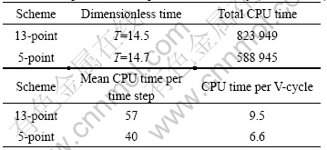
Under the condition of the same convergence criterion and AMG method. The results in Table 2 indicate that the CPU time of new 5-point scheme is less than that of old 13-point scheme and about 3 of CPU time can be saved. In fact, it is because the number of non-zero elements of sparse matrix for 5-point scheme is much less than that of 13-point scheme and then the computational time is down.
4.2 Comparison of computational results
The computational results are compared with each other and also with the experimental data by OKWOUBI and AZAD[8], and SINGH and AZAD[9].The comparisons are shown in Fig.4, Fig.5 and Fig.6 (note: y/D0 is the radial dimensionless coordinate).
From the above comparisons, we can see that under the condition of same numerical experimental environment and computational conditions, the computational precisions of and k have been improved, especially, for turbulence energy k, the computational results in middle position have been greatly improved. For wall static pressure coefficients, the computational results of 5-point scheme agree better with the experimental data than that of 13-point scheme.
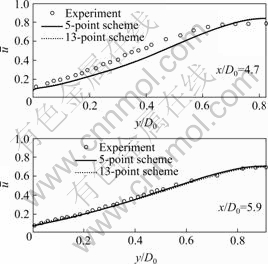
Fig.4 Comparisons of longitudinal velocity profiles: (a) x/D0= 4.7; (b) x/D0=5.9
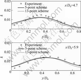
Fig.5 Comparisons of turbulence energy profiles: (a) x/D0=4.7; (b) x/D0=5.9
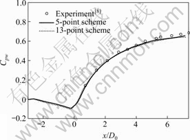
Fig.6 Comparisons of wall static pressure coefficients
5 Conclusions
1) Computational results demonstrate that the proposed method of integrating DLR k-ε turbulence model with algebraic multigrid method is a good way of turbulent numerical prediction.
2) The new 5-point scheme constructed in present work has the dominant advantage over the 13-point scheme.
3) By use of the new 5-point scheme, the precision and efficiency are all improved, especially near the middle position, the precision of computational results for turbulent kinetic energy is obviously improved.
References
[1] JIANG Guang-biao, HE Yong-sen. Study on diagnostic system for numerical prediction of turbulent flow in a conical diffuser: Effect of model functions, grid disposition and Reynolds numbers[J]. Natural Science Journal of Xiangtan University, 2006, 28(2): 1-4. (in Chinese)
[2] HE Yong-sen, LIU Shao-yin. Numerical prediction of turbulent flows in a conical diffuser using k-ε model for near-wall and low Re-number[C]// The 4th Asian International Conference on Fluid Machinery. Suzhou, 1993: 593-599.
[3] HE Yong-sen, LIU Shao-ying. Numerical prediction of turbulent flows through pipelines of machinery[M]. Beijing: National Defence Industry Press, 1999. (in Chinese)
[4] THOMPSON J F, THAMES F C, MASTIN C W. Automatic numerical generation of body-fitted curvilinear coordinate system for fields containing any number of arbitrary two dimensional bodies[J]. J Comp Phys, 1974, 24(5): 299-310.
[5] SHU Shi. Geometry-analysis based algebraic multigrid methods and applications[D]. Xiangtan: Xiangtan University, 2004. (in Chinese)
[6] XIAO Ying-xiong. Study of algebraic multigrid algorithms and applications in solid mechanics[D]. Xiangtan: Xiangtan University, 2006. (in Chinese)
[7] LAUFER J. The structure of turbulence in fully developed pipe flow[M]. Washington: U.S. Government Printing Office, 1955.
[8] OKWUOBI P A C, AZAD R S. Turbulence in a conical diffuser with fully developed flow at entry[J]. J Fluid Mech, 1973, 57(3): 603-622.
[9] SINGH D, AZAD R S. Turbulent kinetic energy balance in a conical diffuser[R]. Manitoba, Canada: Department of Mechanical Engineering University of Manitoba Winniipeg.
(Edited by YANG Hua)
Foundation item: Projects(59375211, 10771178, 10676031) supported by the National Natural Science Foundation of China; Project(07A068) supported by the Key Project of Hunan Education Commission; Project(2005CB321702) supported by the National Key Basic Research Program of China
Received date: 2008-06-25; Accepted date: 2008-08-05
Corresponding author: SHU Shi, Professor, PhD; Tel: +86-732-8293317; E-mail: shushi@xtu.edu.cn

