J. Cent. South Univ. (2018) 25: 2733-2753

DOI: https://doi.org/10.1007/s11771-018-3950-1

Noise comparison of centrifugal pump operating in pump and turbine mode

DONG Liang(董亮)¹, DAI Cui(代翠)^{2, 3}, LIN Hai-bo(林海波)³, CHEN Yi-ping(陈怡平)²

1. Research Center of Fluid Machinery Engineering and Technology, Jiangsu University,Zhenjiang 212013, China;

2. School of Energy and Power Engineering, Jiangsu University, Zhenjiang 212013, China;

3. Sichuan Provincial Key Lab of Process Equipment and Control, Sichuan University of Science & Engineering, Zigong 64300, China

Central South University Press and Springer-Verlag GmbH Germany, part of Springer Nature 2018

Abstract: Investigations regarding the relation of noise performance for centrifugal pump operating in pump and turbine modes continue to be inadequate. This paper presents a series of comparisons of flow-induced noise for both operation modes. The interior flow-borne noise and structure modal were verified through experiments. The flow-borne noise was calculated by the acoustic boundary element method (ABEM), and the flow-induced structure noise was obtained by the coupled acoustic boundary element method (ABEM)/structure finite element method (SFEM). The results show that in pump mode, the pressure fluctuation in the volute is comparable to that in the outlet pipe, but in turbine mode, the pressure fluctuation in the impeller is comparable to that in the draft tube. The main frequency of interior flow-borne noise lies at blade passing frequency (BPF) and it shifts to the 9th BPF for interior flow-induced structure noise. The peak values at horizontal plane appear at the 5th BPF, and at axial plane, they get the highest sound pressure level (SPL) at the 8th BPF. Comparing with interior noise, the SPL of exterior flow-induced structure noise is incredibly small. At the 5th BPF, the pump body, cover and suspension show higher SPL in both modes. The outer walls of turbine generate relatively larger SPL than those of the pump.

Key words: centrifugal pump as turbine; noise performance; acoustic boundary element method; acoustic finite element method

Cite this article as: DONG Liang, DAI Cui, LIN Hai-bo, CHEN Yi-ping. Noise comparison of centrifugal pump operating in pump and turbine mode [J]. Journal of Central South University, 2018, 25(11): 2733–2753. DOI: https://doi.org/10.1007/s11771-018-3950-1.

1 Introduction

Pump is a kind of working machine used to improve the fluid pressure by consuming mechanical energy or other external energy [1]. And the pump can work as an energy generator in reverse direction by recovery of residual fluid pressure, which is also known as pump as turbine (PAT) [2–5]. Due to the advantages of simple structure, low cost of equipment, easy to operate and maintain, pumps and pumps as turbines have been widely applied in many fields from industry to agriculture. To improve the energy conversion efficiency, they are gradually developing towards high-power. Consequently, the increase in power causes large scale of pressure fluctuation, which in turn generates high-level noise.

The flow-induced noise in hydraulic machinery mainly comes from the dipole source acting on the casing walls [6, 7]. And it is excited under the actions of fluid load, structure response and vibroacoustic coupling effect, which is generally characterized by broadband noise with prevailing discrete frequency. In fact, the pressure fluctuation will produce an exciting force on the inner surfaces of casing, which will induce the structural vibration of inner and outer surfaces and the noise radiated inward and outward. Furthermore, the sound wave reacts on the casing in the form of load, thereby generates vibroacoustic coupling effect [8, 9]. According to these, there are two forms of flow-induced noise inside or outside the hydraulic machinery, namely, flow-borne noise and flow-induced structure noise.

Earlier studies in hydraulic machinery, most were focused on exploring the characteristic and mechanism of flow-borne noise purely generated by internal flow in interior field [10, 11]. There are several methods to predict the flow-induced noise in interior field, namely, the acoustic analogy method and the acoustic boundary element method (ABEM). Based on the hypothesis of compact source and low Mach number, the acoustic analogy method is mainly used to predict acoustic at far-field. JEON et al [12] introduced an incompressible two-dimensional discrete vortex method (DVM) to analyze the unsteady flow field of centrifugal fan. Then, using the calculated unsteady force data in the fan flow region, the noise radiations are predicted through FW-H equation. As a physics-based mathematical model used in acoustic software, the acoustic boundary element method (ABEM) can solve the acoustic information of the whole calculation domain without distinguishing near- and far-fields. LIU et al [7] predicted the noise generation within the volute of the centrifugal pump and they employed the newly developed boundary element method. When considering the noise radiated from the structure under the fluid load, the effective coupled method of ABEM and structure finite element method (SFEM) can be adopted. KATO et al [13] and JIANG et al [14] presented a full-scale weakly coupled method for simulating flow-induced noise. Firstly, a time series of pressure fluctuations on inner surface of pump were obtained using CFD program and then they were used for structural analysis based on an explicit dynamic FEM method. However, the final radiated noise from vibration velocity by Sysnoise acoustic software was not involved. KATO et al [15] actually performed the acoustical computation in a multi-stage centrifugal pump, mainly due to rotor-stator interaction. DONG et al [16] solved the exterior flow-induced noises in a centrifugal pump used as turbine by the ABEM and the coupled SFEM/ABEM.

With regards to the exterior noise, the prediction methods of flow-induced structure noise can roughly be classified into two types, namely, analytical method and numerical method [17]. By analytical method, the basic geometry is simplified as simple structure with orthogonal surfaces (such as elastic flat, single or double cylindrical shell, spherical shell, and conical shell) to solve sound parameters using integral transform, modal analysis, wave method, and so on. The method is inappropriate for practical engineering problems although it can effectively reveal the nature of flow-induced structure noise. Based on wave equation, the numerical method can accurately obtain the vibro-acoustic characteristics of complex structure under low- and middle-frequency. When using this method, the structure is commonly discretized by structural finite element method (SFEM), and the acoustic field is processed by acoustic finite element method (AFEM) and acoustic boundary element method (ABEM). The main challenge of exterior noise calculation lies on how to deal with unbounded physical domain. When dealing with acoustic radiation problems in exterior field by ABEM, the derivation of singular Green function integral should be obtained. However, it requires a long time to generate the boundary element matrix. And, without considering the characteristics of various media between interior water and exterior air in pump or PAT, the solution of exterior noise will result in calculation distortion. Relatively, the AFEM is an effective method to calculate exterior noise. XIE et al [18] studied the middle- and low-frequency noise of small-scale stiffened cylindrical shell underwater based on AFEM. It is pointed out that the method is feasible for infinite acoustic field analysis. However, when calculating, the infinite domain should be truncated and the corresponding non-reflecting boundary should be imposed to simulate sound propagation in infinite domain. To make the AFEM satisfy the summerfield radiation condition, ENGQUIST et al [19] introduced artificial boundary condition to truncate the calculation domain. GIVOLI [20] further pointed out when adopting low-order absorbing boundary condition, an extremely large calculation domain will lead to a sharp increase of calculating amount. While, high-order absorbing boundary condition will lower the stability of algorithm. Normally, it is unrealistic to discretize infinite flow domain. Limited truncation is used to substitute unlimited fluid domain by constructing a convex fluid domain surrounding the vibrating structure. There is a problem: smaller truncation can improve computational efficiency with more reflection of sound wave on truncated boundary, whereas, too larger truncation is bound to greatly increase the number of elements, which reduces the efficiency, and even causes the calculation not completeing. Now the problem between computational limit and efficiency is well solved by perfectly matched layer (PML) method. With the development of PML, the automatically matched layer (AML) method can automatically generate matched layer according to finite element model, and change with the frequency to meet the requirement of upper and lower frequency limits. Thus the workload of researcher is greatly reduced, also the computational efficiency is improved.

Note that in those centrifugal pumps and PAT studies, the relations of hydraulic performance between them have been widely and deeply studied; however, different kinds of interior/exterior flow- induced noises are less compared. What is the difference of the flow pattern and noise performance in both pump and modes, and whether there is some relation between them is open for questions.

Here the measurements of interior flow- induced noise and structure modal were conducted. Based on these, the numerical methods of interior/ exterior flow-induced noise in the centrifugal pump and PAT were validated. Eventually, the internal flow comparison was performed to explore the reason of noise performance due to different operation modes. And the noise performance including the spectrum curve and sound pressure distribution of interior/exterior noise was studied.

2 Experimental methodology

2.1 Hydraulic and interior noise measurement

The experimental model is a low-specific speed centrifugal pump with a spiral volute in Ref. [16]. The design parameters of the pump are: flow rate Q_d=52 m³/h, head H_d=18 m, rating speed n=1500 r/min and specific speed n_s=75. The impeller geometrical parameters are β₁=19.5°, β₂=20°, b₂= 14 mm, φ=130°, z=6, D₁=102 mm and D₂=255 mm. The volute geometrical parameters are D₃=266 mm, b₃=26 mm and D₄=65 mm. The rotating speed keeps a constant value of 1500 r/min, so the impeller rotating frequency (APF) is about 25 Hz and the blade passing frequency (BPF) is approximately 150 Hz.

The hydraulic and interior noise measurements of PAT were conducted on a standard test facility in Jiangsu University, as shown in Figure 1. A feed pump was installed to supply high pressure fluid required for impacting the impeller of PAT. An eddy current dynamometer (ECD) was used to consume and measure the energy recovered by PAT. As the core of the entire test, matched with the eddy current dynamometer, the EST measure and control system can make the speed of PAT remain constant over time. The ECD is mainly composed of eddy current brake, force measuring mechanism and correction mechanism. The measured shaft power range is 0–22 kW or 0–118 N·m, with a torque measurement accuracy of ±0.4% F·S and a speed measurement accuracy of (0.1%±1) r /min. Due to the use of indirect water cooling, there is no uncontrollable area of load (only air resistance), so the ECD is quite suitable for the hydraulic performance test for small- and medium-sized PAT at different operating conditions. The discharge and pressure of inlet and outlet were respectively measured by flow meter and pressure transmitter. The measuring range of the flow meter is 20–200 m³/h with an accuracy of ±0.2%. The range of the pressure sensor at inlet is 0.6–1.0 MPa with an accuracy of ±0.1%, while the measured range at outlet is–0.3–0.3 MPa with the same accuracy of ±0.1%. The relative uncertainty of flow rate, head, rotating speed, hydraulic power, shaft power and efficiency is ±0.50%, ±0.14%, 0.07%, ±0.52%, ±1.08% and ±1.20%, respectively, at the best efficiency point (BEP).

Figure 1 Sketch of hydraulic and interior noise test

The sound pressure level (SPL) of PAT was obtained by the INV vibration and noise test system from China Orient Institute of Noise & Vibration. The system consists of INV3020C high- performance 24-position acquisition system and DASP large-capacity data processing software. At present, the methods of detecting the noise characteristic in interior field are indirect test method, lake or sea test method and pipeline test method [21]. The indirect test method indirectly derives the flow-induced noise according to the air-borne sound or the vibration generated during the operation of the equipment. However, due to the complex relationship between the air-borne sound or the vibration and the flow-induced noise, it is difficult to accurately quantify and describe the flow-induced noise. The lake or sea test method can directly measure the noise radiated outward due to the sound source through the pipeline and the port. But it is difficult to implement because of high cost. The pipeline test method can describe the flow- induced noise characteristic by direct using the noise signal measured at a location in the piping system. In this work, a ST70 hydrophone was flush mounted on the outlet piping of PAT, which was arranged at four times outlet diameter. The hydrophone has a frequency range of 50–70×10³ Hz, with a sound pressure sensitivity of –204 dB(re |V| μPa). Since the PAT is placed in a system connected to the pipeline, it is necessary to eliminate the influence of other sources. During the noise measurements, the operating conditions of PAT change by the adjustment of the speed of booster pump with the valves in the loop system remaining fully open, so the impact of valve noise can be ignored. The flush mounted installation of the hydrophone on the inner wall of the pipe can reliably measure the pulsating sound field in the pipeline with the minimized influence on the flow field. The disadvantage of this method is that it is affected by the noise on the wall boundary layer. However, it has been shown that the boundary layer noise is little compared to the pulsating sound when the flow velocity in the pipeline is small [22]. It can be considered that the signal obtained by the hydrophone can reflect the noise radiated by the PAT as a sound source in the specific pipeline. The acquisition frequency was 25.6 kHz with a resolution of 12.5 Hz. To reduce the random noise error, the spectra of four divided pieces of data were averaged, using the whole average method. Besides that, to reduce leakage error in frequency-domain, Hanning window was adopted to process data.

2.2 Model measurement

Based on the excitation and response applied on a system, the modal measurement can describe the dynamic characteristics thorough measurable and controllable dynamic excitation over the structure [23]. In the work, the excitation signal comes from the force sensor mounted on the force hammer, and the response signal comes from the acceleration sensor placed on the casing. By amplifying the collected signals through the signal amplifier, the collected data are transmitted to the dynamic analyzer for analysis. The data analysis and processing is mainly processed by STAR5.0 modal analysis software.

In the paper, the casing was suspended by flexible elastic ropes under free-hanging support, as shown in Figure 2(a). The maximum natural frequency of the test system is much less than 20% of the first-order natural frequency of the casing, so it is in accordance with the free support requirement. The hammering method has the advantages of simple excitation device, easy operation, easy field test and no additional quality and additional restraint. In addition, the hammer strike is a kind of broadband excitation, whose single excitation can stimulate multiple order modes simultaneously. Because the natural frequency of the first few orders of the casing is higher, a wider force spectrum is required, and the hammer is used to produce the excitation signal with a steel head. As the incentive way, the single input single output method is adopted that is constantly moving the incentive points with a single response point fixed. The incentive points should be distributed appropriately to distinguish each order mode of vibration. 306 points were arranged at the main part of casing, as shown in Figure 2(b). For determining the response point, a number of positions on both planes of the bearing box were firstly selected, and then the response effects of these points were tested separately. During the test, the points on six surfaces of the volute were excited to observe the transmission of excitation energy in different directions, with each response signal collected by the three-way acceleration sensor. After the data were collected, they were coherently processed and the spectrum was observed. The coherence function is good, indicating that the excitation energy is better, that is, the response quality is better. Through observing the spectrum, we can generally know the incentive effect of the hammer in certain frequency band. After comparison, the point on the main bearing box was set as the response point, as shown in Figure 2(c). The frequency range of excitation force under normal operating conditions should be considered in the model measurement [24]. The max frequency in the test was 2000 Hz, and the cutoff frequency of general hammer can meet the requirement. The sampling frequency was 5120 Hz with a spectral line number of 800, and then the frequency resolution was 6.4 Hz. In order to ensure that the hammer force is the impulse force, the transient window (force window) was used to improve the signal-to-noise ratio of the excitation signal. Due to short sampling time and slow response attenuation in the test system, the exponential window was adopted to avoid the leakage of frequency response function. Figure 2(d) shows the transfer function of the casing obtained. We can see that for single-point excitation, the excitation signal can be effectively transmitted to the component.

Figure 2 Sketch of model test:

3 Numerical modeling

3.1 Computational fluid dynamics modeling

The fluid domain in whole flow passages, including impeller, volute, leaking chamber, suction pipe and outlet pipe, was discretized with tetrahedral cells, as illustrated in Figure 3. By this, the total hydraulic losses across the impeller and volute were taken into account. With multiple reference frames applied, the flow in the impeller was calculated in a rotating frame, while others were set in stationary frame. Among rotating and stationary domains, the frozen rotor/stator interface was adopted for steady calculation. Apart from the shroud, hub and blade surfaces of the impeller, the inner walls of leaking chamber were set as rotating walls at a speed of 1500 r/min. The no-slip velocity condition was imposed on all wet solid walls with the roughness set to 50 μm. In the pump mode, a pressure-inlet boundary condition was applied at the pump inlet (the suction pipe) where the static pressure level was 1.01325×10⁵ Pa; a mass flow rate-outlet boundary condition was specified at the pump outlet (the outlet pipe) and it rotated in counter-clockwise direction. In the turbine mode, there was a pressure-inlet boundary condition at the turbine inlet (the pump outlet); a mass flow rate-outlet boundary condition was at the turbine outlet (the suction pipe) and it rotated in clockwise direction. The convection items in the turbulence and advection equations were discretized in higher resolution, and the convergence criterion of the residual in those equations was set to 1×10^–5. For sufficiently distinguishing the unsteady information, the time step was set to 1.1111×10^–4 s, which means that the impeller rotates about 1° in each time step [25, 26].

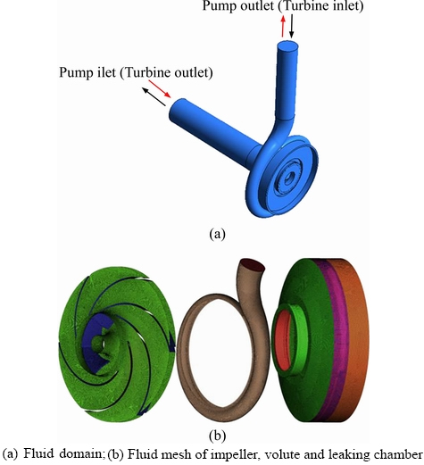
Figure 3 Fluid domains and meshes:

Theoretically, the calculating errors would decrease gradually with an increase of grid number; however, too many grids would pose prohibitive demands on computational resource and time. Three grid sizes were selected to determine the appropriate grid number. Table 1 shows the mesh number of three grid sizes. Among the turbulence models, k–ε and k–ω are known to be the most suitable for internal flow simulation in rotating machines. Therefore, four models, i.e., standard k–ε, RNG k–ε, k–ω and SST k–ω, were selected. The numerical efficiency under different grids and turbulence model in turbine mode were compared with the experimental results, as shown in Table 2. It can be found that, considering the prediction precision and computing time, the standard k–ε model with grid size S2 is more suitable and selected in this study.

Table 1 Mesh number of three grid sizes

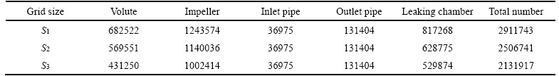
Table 2 Numerical results under different mesh and turbulence models

When focusing on the pressure pulsation characteristics in some important regions, some monitoring points are mounted on the mid-span plane, as illustrated in Figure 4. For the volute, 36 monitoring points (P_v1–P_v36) are circumferential evenly mounted at the volute basic circle with the adjacent angle △α=10°, staring from the tongue. For the impeller, 30 points (P_ip1–P_ip30, P_is1–P_is30) were arranged both on pressure and suction surfaces of blade, starting from r=20 mm with △r=3 mm.And on the inlet pipe, there is one point arranged.

Figure 4 Details of monitoring points on pump/PAT

3.2 Computational acoustics modeling

For the pump or PAT, the noise radiates inside to water and outside to air. Due to the greater acoustic impedance of casing wall than water and air, there is a very small amount of interactive sound transmission between inner and outer wall. So, the vibro-acoustic model can be decoupled in numerical simulation without considering the coupled effect of acoustic radiations in water and air. For the completely vibro-acoustic coupling problems, the wave equation for the structure with hollow space inside is defined as [27]

                   (1)

where M_f, C_f, K_f and R are respectively acoustic equivalent mass matrix, fluid equivalent damping matrix, acoustic equivalent stiffness matrix and coupling matrix of fluid and structure; p is the sound pressure at each node;is the second derivative matrix of node displacement to time.

Ignoring the effect of sound pressure on structure, the control equation for structural vibration is:

                      (2)

where M_s, C_s and K_s are respectively the mass matrix, damping matrix and stiffness matrix of structure; is the displacement vector of structural node; F_s is the external load vector.

Considering the coupled effect of fluid and structure, a surface force will be produced on the interface due to sound pressure. After its transformation onto structural nodes, the control equation for structural vibration becomes

                  (3)

where F_f is the fluid pressure load at the coupled interface.

Equations (1) and (3) are jointly solved to obtain the fluid-structure motion equation under coupling condition

                                (4)

Also, it is the coupled equation of structure and acoustic. As can be seen, the structural vibration will induce sound wave under the effect of load, vice versa, and the radiated sound can cause structural vibration. The displacement and sound pressure on the nodes of structural surface will be obtained by solving Eq. (4). For pump or PAT, the direct solution of equation will take unbearable computational time. The vibration modal is the inherent characteristic of elastic structure. By modal analysis, each order modal characteristic can be found out within a vulnerable frequency band, and then, the real vibration response can be predicted under the external or internal various kinds of vibration source. In this paper, based on structural modal, the vibro-acoustic coupling response will be calculated.

3.3 Interior/exterior acoustics modeling

The flow-borne noise and flow-induced structure noise generated by casing source in interior field of pump and PAT were conducted by ABEM and ABEM/SFEM, respectively. The detail calculation process can be seen in our previous work [16]. The acoustic boundary was meshed with a consistent size of 6 mm, which meets the requirement of calculated frequency, as shown in Figure 5(a). The casing structure used for noise calculation due to structure vibration consists of pump body, cover, suspension, supporting feet, and inlet pipe and outlet pipe. When modeling, it only retains the structures with larger normal radiation area. The other tiny structures, such as the bosses, transition fillets, were removed. Moreover, the holes in structure surface, such as holes for injection and drainage and cover surfaces, were filled. The solid187 was used, and the casing contains 1914480 elements as shown in Figure 5(b). The Gray Cast HT200 was applied, whose density ρ=7200 kg/m³, elastic module E=148 GPa and Poisson ratio μ=0.3. The geometry interpolation method of element maximum distance was adopted to map the acoustic boundary element mesh with the structure finite element mesh. Four closest nodes were interpolated from the elements whose distance was less than 10 mm. To simulate the direct spread of noise in piping without reflection, the inlet pipe and outlet pipe were set as full absorption, and other surfaces were defined as total reflection with the acoustic impedance of 1.5×10⁶ kg/(m²·s). The spectrum for different kinds of flow-induced noise at the same position with the experiment was obtained.

The ABEM is only suitable for the noise problems with one fluid material. Due to internal water and external air in pump and PAT, the AFEM/FFEM was adopted to solve the flow- induced structure noise in exterior field. Considering the vibro-acoustic coupling effect, the pressure fluctuations obtained by flow calculation were firstly imposed on inner walls of casing. Then, the vibration response under fluid load was solved based on structural modal. Finally, with the vibration displacement on outer walls as boundary condition, the exterior noise was solved based on AML. Figures 5(c) and (d) show the acoustic finite element and field point meshes. The mesh contour must be convex to consider the sound interaction between two different domains of vibrating structure. When using the AML method, only the outer surface of finite element enveloping mesh was assigned as AML layer, and the PML layer will be generated automatically inside the solver. The PML layer can be adjusted to comply with the calculation according to computational frequency, which can improve computational accuracy and decrease workload. For acoustic finite element mesh, the internal boundary fitted the shape of casing, and the external convex contour was assigned as AML. The field point mesh of exterior noise was established based on ISO standard. To obtain the distribution of noise, the impeller rotating center (0, 0, 0) was regarded as the origin to establish monitoring planes of 1 m×1 m, respectively, paralleling to x, y, z. These planes were defined as horizontal, vertical, and axial direction. Six monitoring points were disposed on each monitoring plane at 1 m away from the center of impeller, also as shown in Figure 5(d).

Figure 5 Acoustic and structure elements for interior/exterior noise:

4 Results

4.1 Numerical verification

The head, shaft power and hydraulic efficiency curves of pump and PAT are demonstrated in Figure 6(a) as a function of flow rate. The numerical hydraulic performance curves of pump are closer to the experimental curves. The shaft power shows the biggest error of 3.89% at 80 m³/h. The hydraulic efficiency shows bigger error at larger flow rate with the biggest error of 3.10%, while the head shows bigger error at smaller flow rate with the biggest error of 3.48%. The hydraulic performance curves of PAT show similar trends with those obtained by the experiment, especially at flow rates larger than 90 m³/h. The BEP of pump and turbine is respectively nearly at 60 m³/h and 90 m³/h.

The spectra curves in interior filed of PAT are compared with the experiment at 90 m³/h, as shown in Figure 6(b). It is found that the calculated spectrum curves obtained from flow-borne noise due to casing source are in good agreement with the experiment. Within the range below 450 Hz, larger differences at broadband exist, and the experimental value is higher than the calculated value on the whole. The predicted values show similar pattern and consistent deviation in terms of magnitude with the acoustics experiment. The causes of error may be that the impeller with certain dynamical unbalance generates certain levels of vibration at the hydrophone, which lowers the measurement accuracy. And the stronger swirling flow of PAT enlarges the calculated error based on URANS.

Figure 6 Hydraulic performance and interior noise curves in pump and turbine modes:

During the modal simulation of the casing, the prestress is not applied in the solution process. Table 3 gives the first six modal frequencies in free condition. And, Figure 7 shows the corresponding vibration models. As can be seen, the modes of vibration are approximate between the calculation and experiment. The calculated errors of modal frequencies are within 7%, which means that the finite element model is available to noise analysis based on the vibration modal. In practice, the pump or PAT was fixed on ground by bolts, and the inlet and outlet were connected with inlet pipe and outlet pipe. So the boundary conditions of modal analysis for the casing were set as the bottom contacted with ground was supposed six constraints of x, y and z directions; the up and down displacement were restricted on the pump outlet (turbine inlet) pipe; the axial displacement was restricted on the pump inlet (turbine outlet) pipe. The first 8-order constraint natural frequencies were 311.10, 416.83, 762.87, 886.73, 1363.75, 1603.67, 1715.77 and 1919.75 Hz, respectively.

Table 3 Comparison of free modal frequency between calculation and experiment

4.2 Internal flow comparison of pump and turbine

The fluid streamlines through the whole flow passages are illustrated in Figure 8 in pump and turbine modes. We can see that in the suction pipe of the low-specific speed centrifugal pump, the fluid axially flows into the impeller at all flow rates. While, it exhibits a strong swirling flow in the draft tube of turbine, whose rotational direction is positive to the impeller. The generated circumferential component of velocity would produce an extra skin friction loss to augment the total hydraulic loss in the draft tube. On the other hand, it would aggravate the fluctuation of pressure. In the same case, there is a swirling flow in the outlet pipe of pump, and the degree increases with increasing flow rate, showing the enlarged circumferential velocity in magnitude.

For comprehensively understanding the unsteady pressure fluctuation (C_p) in the impeller, volute, inlet pipe and outlet pipe in pump and turbine modes, Figure 9 shows the pressure fluctuation spectra of monitoring points at their BEPs.

It is observed in pump mode that the spectra at the monitoring points of the volute and outlet pipe (P_vp1, P_op1) present typical prevailing discrete frequency. The peak value mainly appears at BPF and its higher harmonics, and the amplitude at BPF is much larger than that at higher harmonics. Thus, the rotor-stator interaction effect is the dominant source of pressure fluctuations in the volute and outlet pipe. It is noted that the amplitudes in the spectrum at point P_op1 are smaller than those at point P_vp1, i.e., the amplitude at BPF is decreased by 58.4%, indicating that the pressure fluctuation in the outlet pipe is mainly induced by the transmission of that in the volute. While at the points in the impeller (P_ipp1, P_ips1), the peak values mainly appear at APF, BPF and their higher harmonics, with lots of other peak frequencies (262.5 Hz, 287.5 Hz and so on) induced by nonlinear interference between APF and BPF. The amplitude at APF is much larger than other frequencies, i.e., the amplitudes at APF are 7.2 and 2.9 times that at BPF. While compared with the pressure fluctuation in the volute and outlet pipe, the amplitudes in the impeller is dramatically lower. It is indicated that the pressure fluctuation in the impeller mainly comes from the rotation of impeller, and the transmission due to the rotor-stator interaction in the volute is not obvious. At the suction pipe, the pressure fluctuation is extremely low, mainly because a liquid is sucked into the suction pipe without any pre-swirl as shown in Figure 8(b).

Figure 7 Comparison of free vibration modal between calculation and experiment:

Figure 8 Fluid streamlines in pump and turbine mode:

Figure 9 Pressure fluctuation spectra of monitoring points in pump and turbine modes at BEPs:

In turbine mode, the liquid exhibits a clockwise circulation at the exit of volute and impacts the blades to put the impeller into rotation and eventually discharge out of the turbine from the draft tube. Among all the flow passage components, the pressure fluctuation in the impeller (P_itp1, P_its1) is the most strong in PAT and its main frequency is located at BPF rather than APF. All these can be inferred the pressure fluctuation due to the rotor-stator interaction tending to propagate downstream. At the monitoring point of the volute and draft tube (P_vt1, P_dt1), the pressure fluctuation displays typical spectrum chartered by discrete frequencies of BPF and their harmonics. However, in the draft tube, the amplitude at BPF is higher than that in the volute, which further proves the ease transmission downstream rather than upstream. On the other hand, from Figure 8(e), there is a strong swirling flow in the draft tube of turbine, which may increase the pressure fluctuation. At the inlet pipe of turbine, due to a relative smooth flow, the pressure fluctuation is weaker with no peak values.

In the volute, the amplitude at BPF dominates the energy of the spectrum in pump and turbine modes. Figure 10 gives the amplitude distribution at BPF in circumferential direction at different flow rates. From Figure 10(a), we can that see in pump mode, the circumferential distribution of pressure fluctuation at BPF presents a typical six peaks at three flow rates, implying that it is caused by the rotor-stator interaction between the impeller and the tongue. At the BEPs and small flow rates, the maximum value is located at the tongue θ=0°, while it appears at θ=10° at the large flow rate. As we know, the intensity of rotor-stator interaction is mainly determined by the impinging effect on the tongue due to the blade wake. When the wake interacts with the tongue, the more intense turbulent flow structure will generate near the region, which will result in a larger magnitude of pressure fluctuation. At three flow rates, the amplitude of monitoring point basically goes down with the increasing angle, which may be induced by the increasing radial gap between the impeller and volute. Compared with small and large flow rates, the change rate of the amplitude becomes weaker in circumferential direction at BEPs (except θ=0°), mainly due to the uniform flow discharging from the impeller. It is interesting to notice that, the peak and trough of the amplitude at the small flow rate are nearly opposite with that of the BEPs and large flow rates.

Figure 10 Amplitude distribution at BPF in circumferential direction in volute in pump and turbine modes at different flow rates:

From Figure 10(b), in turbine mode, the periodic feature with six peaks is also observed caused by the presence of six blades. What is difference, the amplitude at the peak basically ascends with the increasing angle, and the maximum value lies at θ=310°, 320° and 330° respectively for 80, 90 and 110 m³/h. That is to say, the rotor-stator interaction effect on the zone is stronger. And with the increase of flow rate, the amplitude at BPF of pressure fluctuation increases. As we know, apart from BPF, there are still other harmonic frequencies, so the total energy of the pressure spectrum should be the sum of the discrete frequencies. Although the amplitude at BPF plays a dominant role in the pressure spectrum of volute, it only represents part of the energy in the whole spectrum. This is probably why the amplitude at BPF ascends with the increase of flow rate.

In the impeller, the amplitude at APF and BPF respectively dominate the energy of the spectrum in pump and turbine modes. Figure 11 gives the amplitude distributions of pump at APF and the amplitude distribution of turbine at BPF on pressure and suction surfaces at different flow rates. We can see that in the pump mode, the amplitude on the pressure surface firstly increases and then decreases at 40 m³/h and 60 m³/h. The maximum value is located at the trailing edge, that is r=104 mm for 40 m³/h and r=92 mm for 60 m³/h. However, the amplitude on the pressure surface basically remains unchanged at 80 m³/h. It is interesting to notice that the amplitude at higher flow rate is the lowest compared with the other flow rates. However, on the suction surface, the amplitude gradually increases with the increasing radius, and it is most significant at 80 m³/h than those at other flow rates. All these indicate that at larger flow rate, the inner flow in the blade is more complex. In the turbine mode, at 80 m³/h and 90 m³/h, the amplitude on the pressure surface gradually lowers, and it presents a little change on the suction surface. And at 110 m³/h, it changes dramatically on both the pressure and suction surfaces, implying that the pressure fluctuation is sensitive to the higher flow rate.

Figure 11 Amplitude distribution at APF and BPF in impeller respectively in pump and turbine modes at different flow rates:

To disclose the underlying mechanism, the velocity streamlines in the mid-span plane of the impeller and volute at tree flow rates are demonstrated in Figure 12. As we see, the velocity distribution of the pump is relatively uniform, and there is a phenomenon of jet wake at the impeller outlet. A disturbance flow generates near the tongue with the impact of the jet wake. And the degree of disturbance lowers in the volute with incensement of angle, which indicates the amplitude of pressure fluctuation is larger at zone B. And it is consistent with the amplitude distribution of pump at BPF in circumferential direction in the volute as shown in Figure 10(a). In the turbine mode, when the flow rate is below 90 m³/h, the liquid impinges the blade suction surface directly, causing a flow separation from the blade pressure surface in the most portion of blade. As the flow is above 90 m³/h, there is a larger reverse flow zone at most portion of suction surface of blade and a relative small vortex near the rear edge of the pressure surface. At 90 m³/h, even though the liquid can flow into the impeller smoothly, the fluid still separates from the pressure surface of blade in the rear portion of blade. The flow separation disturbs the spread of pressure fluctuation at BPF, especially at larger flow rates, as shown in Figures 11(c) and (d). And the range and intensity of flow separation zone at zone A is greater than the other zones, which reveals that the amplitude in the volute is relatively larger at zone A as shown in Figure 10(b).

4.3 Interior noise comparison of pump and turbine

The spectrum curves of interior noise at pump inlet and turbine outlet are demonstrated in Figure 13 at their BEPs. The sound pressure levels (SPLs) are obtained with respect to the reference sound pressure of 20 μPa.

From Figure 13(a), we can see the main frequencies of interior flow-borne noise both in pump and turbine lie in BPF and its harmonics, suggesting that the main factor affecting the flow-borne noise is the interaction between the impeller and tongue. At the turbine outlet, the SPLs at main frequencies are basically higher than those at the pump inlet. For example, the SPL at BPF at the turbine outlet is 2.5 times that at the pump inlet. And, the broadband noise at the turbine outlet shows wider and higher values than that at the pump inlet. The reason for this is that there is swirling flow in the draft tube of turbine even at BEP as shown in Figure 8(e), which forms additional velocity and pressure fluctuations.

Figure 12 Velocity streamlines in mid-span plane of impeller and volute in pump and turbine modes at different flow rates:

In Figure 13(b), the flow-induced structure noise from pump and turbine is characterized by broadband noise with prevailing discrete frequency tones. And the SPLs at main discrete frequencies of turbine are comparable to those in pump. The broadband noise of turbine is more noticeable in sound spectrum especially in the frequencies higher than 1300 Hz, i.e., the 9th BPF. Compared with the flow-borne noise, the SPLs at discrete or broadband frequencies both in pump and turbine are lower due to flow-induced structure noise, with the biggest decline of 60 dB in pump, suggesting that part of the sound energy is dissipated by the casing vibration. And it can be inferred that the flow- induced structure noise is not leading in interior noise. The dominant frequency shifts to the 9th BPF, whose SPL is 114.00 dB in pump and 124.42 dB in turbine. This is because the vibration response is easily excited when the frequency is close to the 5-order constraint frequency of casing.

Figure 13 Spectrum curves of interior noise at pump inlet (turbine outlet) at BEPs:

The sound pressure distributions of interior noise in pump and turbine are presented in Figure 14 at their BEPs. Due to the fact that the dominant frequencies of interior flow-borne noise and interior flow-induced structure noise are respectivly BPF and the 9th BPF as shown in Figure 13, the sound pressure is distributed at the consistent frequencies. At BPF, in pump, the sound pressure within the whole interior field is comparable in magnitude. However, in turbine, most of the sound energy radiated due to flow-borne noise is concentrated on the walls of casing and draft tube, indicating that these locations have strong noise radiation ability. The turbine inlet pipe shows relatively small sound pressure of about 140 dB. Note that at corresponding locations, the sound pressure in turbine mode is always more substantial than in pump mode, especially at the draft tube (suction pipe of pump), suggesting that there is a more intense unsteady flow in turbine as shown in Figures 8(b) and (e). In terms of flow-induced structure noise at the 9th BPF, the sound pressure distribution in pump mode can be found inhomogeneous, even in the suction pipe or outlet pipe. And the whole sound pressure distribution in turbine mode is quite similar to that in pump. Further in both modes, the whole sound pressure due to flow-borne noise is higher than that of flow-induced structure noise. All these imply that the structural vibration under fluid load not only weakens the SPLs at certain frequencies, but changes the sound pressure distribution inside the casing.

Figure 14  Sound pressure distribution of interior noise at BEPs:

4.4 Exterior noise comparison of pump and turbine

The spectrum curves of exterior flow-induced structure noise in pump and turbine are demonstrated in Figure 15 at their BEPs. It is shown that the SPLs of M1, M2, M3 and M4 at horizontal plane are basically equivalent. The peak value occurs at the 5th BPF, mainly because they are close to 3-order constraint frequency of casing, which causes certain resonance between fluid and structure. On the other hand, it can be inferred that the exterior noise can be determined both by internal pressure fluctuation and structure. At the 5th BPF, the average SPL at the four monitoring points is about 56.85 dB in pump mode, while it is 58.32 dB in turbine mode. At other discrete and broadband frequencies, the SPLs in turbine mode are larger. For the spectrum curves of M5 and M6 at axial plane (see Figures 15(e) and (f)), they show similar tendency, and get the highest SPL at the 8th BPF. At the 8th BPF, the average SPL at the two monitoring points is about 61.53 dB in pump mode, while it is 74.71 dB in turbine mode. Comparing with interior noise in Figure 13, the SPL induced by exterior flow-induced structure noise is incredibly small, indicating that the structure isolates most of internal sound energy.

The sound pressures on the exterior field under the exterior flow-induced structure noise in pump and turbine are distributed in Figure 16 at their BEPs. We can see that at the 5th BPF, the pump body, cover and suspension show higher SPL in both modes. The outer walls of turbine generate relatively larger pressure amplitude than those of the pump. It is interesting to notice that on the exterior field, the sound pressure radiated from the pump is considerable larger compared with the turbine. The SPL on the exterior field mesh of turbine remains 35.7 dB to 63 dB, while the SPL of pump remains 29.4 dB to 88.5 dB. In a similar pattern, at the 8th BPF, the sound pressure distribution on the outer walls of turbine is comparable with that of the pump. Still strange, the sound pressure distribution on the exterior field mesh of turbine is much smaller in magnitude than that on pump.

Figure 15 Spectrum curves of exterior noise at six monitoring points at BEPs:

5 Conclusions

In the study, after confirming the numerical methods of noise prediction, the difference of interior/exterior noise of centrifugal pump operating in pump and turbine modes was emphatically investigated.

In the pump mode, the peak values at the monitoring points of the volute and outlet pipe appear at BPF and their higher harmonics. And the amplitudes in the outlet pipe are smaller than those in the volute. In the impeller, the peak values mainly appear at APF and BPF, with lots of other peak frequencies induced by nonlinear interference between APF and BPF. Compared with the pressure fluctuation in the volute and outlet pipe, the amplitudes in the impeller are dramatically lower. In turbine mode, the pressure fluctuation in the impeller is most strong in turbine and its main frequency is located at BPF rather than APF. At the volute and draft tube, the pressure fluctuation displays typical spectrum chartered by discrete frequencies of BPF and their harmonics. However in the draft tube, the amplitude at BPF is higher than that in the volute, which further proves the ease transmission downstream rather than upstream. The circumferential distribution of pressure fluctuation at BPF presents a typical six peaks at three flow rates. In the impeller, the amplitude at APF and BPF respectively dominates the energy of the spectrum in pump and turbine modes. All these are connected with the velocity streamlines of the impeller and volute in both modes.

Figuer 16 Sound pressure distribution of exterior noise at BEPs:

The main frequencies of interior flow-borne noise both in pump and turbine lie in BPF, and the SPL at the turbine outlet is basically higher than that at the pump inlet. The SPLs at main frequencies of flow-induced structure noise in turbine are comparable to those in pump. Compared with the flow-borne noise, the SPLs at discrete or broadband frequencies both in pump and turbine are lower due to flow-induced structure noise. The dominant frequency shifts to the 9th BPF. At BPF, in pump, the sound pressure within the whole interior field is comparable in magnitude. However, in turbine, most of sound energy radiated due to flow-borne noise is concentrated on the walls of casing and draft tube. And the whole sound pressure distribution in turbine mode is quite similar to that in pump. In both modes, the whole sound pressure due to flow-borne noise is higher than that of flow-induced structure noise.

For the exterior flow-induced structure noise in pump and turbine, the SPLs of M1, M2, M3 and M4 at horizontal plane are basically equivalent. The peak value occurs at the 5th BPF, mainly because they are close to 3-order constraint frequency of casing. For the spectrum curves of M5 and M6 at axial plane, they show similar tendency, and get the highest SPL at the 8th BPF. At the 5th BPF, the pump body, cover and suspension show higher SPL in both modes. The outer walls of turbine generate relatively large pressure amplitude than those of the pump. The sound pressure radiated from the pump is considerable larger compared with the turbine. At the 8th BPF, the sound pressure distribution on the outer walls of turbine is comparable with that of the pump. The sound pressure distribution on the exterior field of turbine is much smaller in magnitude than that on pump.

Nomenclature

a

Coefficient related to volute shape

A

Area of impeller inlet or outlet, mm²

b

Impeller width, mm

b₃

Volute outlet width, mm

D

Impeller diameter, mm

D₃

Volute base circle diameter, mm

D₄

Volute outlet diameter, mm

f

Area-averaged skin friction factor

g

Acceleration due to gravity, 9.81 m/s²

h

Total hydraulic loss, m

H

Head, m

n

Rotating speed, r/min

n_s

Specific speed

P

Shaft power, kW

P_m

Power loss due to mechanical friction, kW

P_l

Power loss due to volumetric leakage, kW

Q

Flow rate, m³/h

s

Static moment of line to rotating axis in peripheral projection, N·m

S

Sensitivity coefficient

u

Impeller tip speed, m/s

v

Fluid absolute velocity, m/s

x₀

Geometry parameter of initial model

Δx

Change of geometry parameters among different models

y₀

Hydraulic efficiency of initial model

Δy

Change of hydraulic efficiency among different models

z

Blade number

Greek symbols

α

Absolute flow angle, (°)

β

Blade angle or relative flow angle, (°)

η_h

Hydraulic efficiency, %

ξ

Total hydraulic loss coefficient

ρ

Fluid density, kg/m³

σ

Slip factor

τ

Average shear stress, Pa

φ

Blade wrap angle, (°)

ψ

Empirical coefficient

References

[1] ZHANG H, DENG S, QU Y. Differential amplification method for flow structures analysis of centrifugal pump between design and off-design points [J]. Journal of Central South University, 2017, 24(6): 1443–1449.

[2] SINGH P, NESTMANN F. An optimization routine on a prediction and selection model for turbine operation of centrifugal pumps [J]. Experimental Thermal and Fluid Science, 2010, 34(2): 152–164.

[3] JAIN S, PATEL R. Investigations on pump running in turbine mode: A review of the state-of-the-art [J]. Renewable and Sustainable Energy Reviews, 2014, 30(2): 841–868.

[4] WANG T, WANG C, KONG F Y, GUO Q Q, YANG S S. Theoretical, experimental, and numerical study of special impeller used in turbine mode of centrifugal pump as turbine [J]. Energy, 2017, 130: 473–485.

[5] DOSHI A, CHANNIWALA S, SINGH P. Inlet impeller rounding in pumps as turbines: An experimental study to investigate the relative effects of blade and shroud rounding [J]. Experimental Thermal Fluid Science, 2017, 82: 333–348.

[6] DAI Cui. Theoretical, numerical and experimental research on fluid-induced noise characteristics for centrifugal pump as turbine [D]. Zhenjiang: Jiangsu University, 2015. (in Chinese)

[7] LIU H L, DAI H W, DING J, TAN M G, WANG Y, HUANG H Q. Numerical and experimental studies of hydraulic noise induced by surface dipole sources in a centrifugal pump [J]. Journal of Hydrodynamics, 2016, 28(1): 43–51.

[8] ZHOU H H, MAO Y J, ZHANG Q L, ZHAO C, QI D T, DIAO Q. Vibro-acoustics of a pipeline centrifugal compressor part I. Experimental study [J]. Applied Acoustics, 2018, 31: 112–128.

[9] ZHANG Q L, MAO, Y J , ZHOU H H, ZHAO C, DIAO Q, QI D T. Vibro-acoustics of a pipeline centrifugal compressor Part II. Control with the micro-perforated panel [J]. Applied Acoustics, 2018, 132: 152–166.

[10] SHEN X, AVITALA E, ZHAO Q H, GAO J H, LI X D, PAUL G, KORAKIANITIS T. Surface curvature effects on the tonal noise performance of a low Reynolds number aerofoil [J]. Applied Acoustics, 2017, 125: 34–40.

[11] PARAMASIVAM K, RAJOO S, ROMAGNOLI A, YAHYA W J. Tonal noise prediction in a small high speed centrifugal fan and experimental validation [J]. Applied Acoustics, 2017, 125: 59–70.

[12] JEON W H, LEE D J. A numerical study on the flow and sound fields of centrifugal impeller located near a wedge [J]. Journal of Sound and Vibration, 2003, 266(4): 785–804.

[13] KATO C, YOSHIMURA S, YAMADE Y, JIANG Y Y, WANG H, IMAI R, KATSURA H, YOSHIDA T, TAKANO Y. Prediction of the noise from a multi-stage centrifugal pump [C]// ASME 2005 Fluids Engineering Division Summer Meeting. Houston, USA, 2005: 19–23.

[14] JIANG Y Y, YOSHIMURA S, INAI R, KATSURA H, YOSHIDA T, KATO C. Quantitative evaluation of flow-induced structural vibration and noise in turbomachinery by full-scale weakly coupled simulation [J]. Journal of Fluids and Structures, 2007, 23(4): 531–544.

[15] KATO C, YAMADE Y, WANG H, GUO Y, MIYAZAWA M, TAKALSHI T, YOSHIMURA S, TAKANO Y. Numerical prediction of sound generated from flows with a low Mach number [J]. Computers & Fluids, 2007, 36(1): 53–68.

[16] DONG L, DAI C, LIU H L, KONG F Y. Experimental and numerical investigation of interior flow-induced noise in pump as turbine [J]. Journal of Vibroengineering, 2016, 18(5): 3383–3396.

[17] GAO M, DONG P X, LEI S H, TURAN A. Computational study of the noise radiation in a centrifugal pump when flow rate changes [J]. Energies, 2017, 10(2): 221.

[18] XIE Zhi-yong, ZHOU Qi-dou, JI Gang. Computation and measurement of double shell vibration mode with fluid load [J]. Journal of Naval University of Engineering, 2009, 21(2): 97–101. (in Chinese)

[19] ENGQUIST B, MAJDA A. Absorbing boundary conditions for numerical simulation of waves [J]. Proceedings of the National Academy of Sciences, 1977, 74(5): 1765–1766.

[20] GIVOLI D. High-order local non-reflecting boundary conditions: A review [J]. Wave Motion, 2004, 39(4): 319–326.

[21] FENG T. The measurement study of the flow-induced noise in centrifugal pumps [D]. Beijing: Institute of Acoustics, Chinese Academy of Sciences, 2005. (in Chinese)

[22] WANG T, LIU K, LI Xiao-hong, TONG Xiao-peng. Development of the experimental system for measuring the hydrodynamic noise in centrifugal pump [J]. Fluid Machinery,2005, 33(4): 27–30. (in Chinese)

[23] ZHANG Y X, LIU X, CHU Z G, HHUANG D, WANG G J. Autonomous modal parameter extraction based on stochastic subspace identification [J]. Journal of Mechanical Engineering, 2018, 54(9): 187–194.

[24] DU Y. The experimental modal analysis method’s applications in surface grinder type msy7115 and its dynamic modification [D]. Kunming: Kunming University of Science and Technology, 2002. (in Chinese)

[25] DAI C, KONG F Y, DONG L. Pressure fluctuation and its influencing factor analysis in circulating water pump [J]. Journal of Central South University, 2013, 20(1):149–155.

[26] WU D, JIANG X, CHU N, WU P, WANG L. Numerical simulation on rotordynamic characteristics of annular seal under uniform and non-uniform flows [J]. Journal of Central South University, 2017, 24(8): 1889–1897.

[27] SHANG D J, HE Z Y. The numerical analysis of sound and vibration from a ring-stiffened cylindrical double-shell by FEM and BEM [J]. Acta Acustica, 2001, 26(3): 193–201.

(Edited by YANG Hua)

中文导读

离心泵与透平运行工况的噪声对比

摘要：离心泵在泵与透平运行工况下噪声性能关联关系的研究还不充分，本文对两种工况下的流体诱发噪声特性进行对比研究。在试验验证内部流动噪声和结构模态准确性的基础上，采用声边界元法（ABEM）计算流动噪声，采用声边界元/结构有限元耦合法（ABEM/SFEM）计算流激结构声。结果表明，在泵工况下，蜗壳内的压力脉动水平与出口管相当；但在透平工况下，叶轮内的压力脉动水平与尾水管相当。内场流动噪声的主频为叶频，而内场流激结构声的主频为9倍叶频。对于外场噪声，水平面上的噪声峰值出现在5倍叶频，而轴面上的峰值出现在8倍叶频。与内场噪声相比，外流流激结构声的声压级相当小。对于两种工况，泵体、泵盖和悬架在5倍叶频处都辐射出较高的声压级；而透平工况下的外壁面辐射出的声压级相对较大。

关键词：离心泵与透平；噪声性能；声边界元法；声有限元法

Foundation item: Project(51509111) supported by the National Natural Science Foundation of China; Project(2017M611721) supported by the China Postdoctoral Science Foundation; Project(BY2016072-01) supported by the Association Innovation Fund of Production, Learning, and Research, China; Projects(GY2017001, GY2018025) supported by Zhenjiang Key Research and Development Plan, China; Projects(szjj2015-017, szjj2017-094) supported by the Open Research Subject of Key Laboratory of Fluid and Power Machinery, China; Project(GK201614) supported by Sichuan Provincial Key Lab of Process Equipment and Control, China; Project supported by the Priority Academic Program Development of Jiangsu Higher Education Institutions (PAPD), China

Received date: 2018-04-28; Accepted date: 2018-08-31

Corresponding author: DAI Cui, PhD, Associate Professor; Tel: +86-18352859360; E-mail: daicui@ujs.edu.cn; ORCID: 0000-0001- 6965-7906