J. Cent. South Univ. (2012) 19: 1454-1465

DOI: 10.1007/s11771-012-1162-7

Vision-based long-distance lane perception and front vehicle location for full autonomous vehicles on highway roads

LIU Xin(刘欣), XU Xin(徐昕), DAI Bin(戴斌)

Institute of Automation, National University of Defense Technology, Changsha 410073, China

? Central South University Press and Springer-Verlag Berlin Heidelberg 2012

Abstract: A new vision-based long-distance lane perception and front vehicle location method was developed for decision making of full autonomous vehicles on highway roads. Firstly, a real-time long-distance lane detection approach was presented based on a linear-cubic road model for two-lane highways. By using a novel robust lane marking feature which combines the constraints of intensity, edge and width, the lane markings in far regions were extracted accurately and efficiently. Next, the detected lane lines were selected and tracked by estimating the lateral offset and heading angle of ego vehicle with a Kalman filter. Finally, front vehicles were located on correct lanes using the tracked lane lines. Experiment results show that the proposed lane perception approach can achieve an average correct detection rate of 94.37% with an average false positive detection rate of 0.35%. The proposed approaches for long-distance lane perception and front vehicle location were validated in a 286 km full autonomous drive experiment under real traffic conditions. This successful experiment shows that the approaches are effective and robust enough for full autonomous vehicles on highway roads.

Key words: lane detection; lane tracking; front vehicle location; full autonomous vehicle; feature line section; autonomous driving; vision

1 Introduction

Intelligent vehicles running on highway roads have been researched since the late 1980s with the increasing demands for transportation and safety. Lane information detected by sensors is required by many integrated applications of intelligent vehicles [1], such as lane departure warning [2-4], adaptive lane keeping [5], driver attention monitoring [6], driver intent prediction [7] and automatic vehicle control [8]. As an indispensable component of an intelligent vehicle, lane detection algorithms extract lane markings from road images to generate lane lines as the guard lines and the safe boundaries of the vehicle.

In most of previous works, lane detection was completed by vision only. A wide variety of vision-based lane detection algorithms with various lane representations have been studied [8-18]. Vision-based lane detection algorithms often represent the road as a mathematical model, such as straight line [8], clothoid [9], B-spline [10], hyperbola [11] and parabola [12]. Then, the road models are fitted by using lane marking features extracted from the road images. There are a wide variety of low-level features used in previous studies, such as corners [13], edges [8-10], colors [14] and textures [15].

McCall and TRIVEDI [5] used an approximately parabolic model with the assumption of flat roads for lane representation and steerable filters were employed for robust and accurate lane-marking detection. The steerable filters provided an efficient method for extracting a wide variety of lane markings under varying lightening and road conditions. WANG et al [16] presented a robust lane detection and tracking method based on a hyperbolic road model and a condensation particle filter. Geometrical and statistical reasoning in vanishing point detection was utilized to accurately estimate the parameters of the road model.

Since long-distance lane information is insignificant for some applications such as active braking systems, many lane detection algorithms are only focused on detecting the lanes in near regions, which are usually no more than 60 m away. However, it is very important for full autonomous vehicle to detect lane information in a long distance. As the most intelligent vehicle, a full autonomous vehicle not only needs to run automatically by following the lanes, but also needs to have the functions of car following, lane changing and autonomous overtaking. When a vehicle appears in front of the autonomous vehicle, some fatal decisions should be made in time: to follow the front vehicle or overtake it; to change the lane or not (see Fig. 1). At this time, the front vehicle must be correctly located on a lane as far as possible to support the decision-making process. In order to complete the above real-time decision-making task, extracting lane information in long distance is the most important and reliable way.

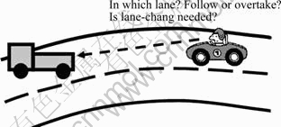
Fig. 1 Full autonomous vehicle to locate front vehicle on correct lane in long distance

Nowadays, laser or millimeter-wave radars are more and more used in full autonomous vehicles so that front vehicles can be detected up to 120 m away [19-20]. So, it is desirable to detect lane markings at the same distance to determine its driving strategy and actions. However, according to our best knowledge, little work has been done on long-distance lane detection. Therefore, the aim of this work is to present a real-time long-distance lane detection approach to meet this requirement based on a linear-cubic road model for two-lane highways as well as a novel lane marking feature. The lane marking feature combines the constraints of intensity, edge and width, simultaneously. Based on this feature, lane markings in far regions are extracted accurately and efficiently. Then, the ego vehicle lateral offset and heading angle can be computed for lane tracking. The detected lane lines are selected and tracked by estimating the lateral offset and heading angle of the ego vehicle using a Kalman filter. Finally, the front vehicles are located on the correct lane using the tracked lane lines. The flow chart of the whole algorithm is shown in Fig. 2.

The proposed approaches were implemented as a main module of the novel “road environment perception system” (REPS) designed for the HQ3 full autonomous vehicle (HQ3-FAV), a new generation full autonomous vehicle running on highway roads. The effectiveness of the proposed approaches was validated in a 286 km full autonomous drive experiment under real traffic conditions.

2 Road model

There are usually two or more lanes on highway roads. In this work, only a two-lane road model is considered to simplify notations. The two-lane road model contains three lane lines: two solid boundary lines and a segmented line in the middle. The three lane lines are parallel, and the distance between two lines is fixed.

Fig. 2 Flow chat of proposed lane perception method

By approximating the clothoid model commonly used in the construction of highway roads, a parabola model can provide sufficient road information: position, angle and curvature, while it is simple enough for computation. However, when a parabolic model is used in long-distance lane detection, the detection error of far lane markings often causes fitting errors of lane lines in near regions.

JUNG and KELBER [17] presented a linear-parabolic road model that represents the lane line as a straight line in near region and a parabolic curve in far region. In the linear-parabolic road model, the straight line is fitted just by the lane markings in near regions and it will not be affected by the detection error of far lane markings. In addition, the parabolic curve can still provide the curvature of the road. Nevertheless, it is noticed that large fitting errors in far regions might occur on many occasions in practice. This means that the accuracy is not enough to fit the lane line in far regions as a parabolic curve since the road is not flat everywhere.

Using cubic curves instead of parabolic curves, a linear-cubic road model is presented in this work to decrease the fitting errors in the far region (see Fig. 3).

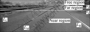
Fig. 3 Linear-cubic road model

The point P(u_x, v_x) in lane line L_x satisfies:

   (1)

where x∈{L, M, R}, denotes which lane line is referred to. The parameters v_n and v_f divide the camera view field into three regions: the near region, the far region and the free region. Here, v_f is fixed while v_n is variable. The parameter v_f is set as a value corresponding to the 120 m distance and it is computed using camera calibration data in initialization. The parameter v_n is computed for near regions which are 30-60 m away and it is adaptive with the curvature of the lane line. The parameters α and β represent the linear part of the lane line in near regions, and γ and λ are related to the curvature of the lane line in far regions.

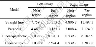
The comparison among different models is shown in Fig. 4. The standard deviations of the fitting errors of the right boundary line in the near and far regions of the two images in Fig. 4 are listed in Table 1. The features for model fitting use the same set of lane marking features. The results of model fitting indicate that the fitting error of the linear-cubic model is smaller than that of other models. Especially, compared with the linear-parabolic model, the fitting error of the linear-cubic model is decreased greatly in the far region, although the fitting errors of the two models in the near region are completely same.

3 Lane detection

3.1 Feature line section

The road model can be fitted with lane marking features extracted from the road images, such as corners, edges, colors and texture. But the direct relationship between these features and the lane markings is hard to be established because these features exist not only in lane marking regions of the input image, but also in background regions. Researchers have to use complex and computationally expensive methods to organize these features to generate the lane line, such as Hough Transform [4] or RANSAC [18]. But for high-speed autonomous vehicles on highways, neither the effectiveness nor the efficiency of these methods is satisfactory.

To solve this problem, a specific feature, which exists only in lane marking regions of input images, needs to be defined for lane detection according to the uniqueness of the lane markings. This means that some prior knowledge about lane markings must be used in feature definition. Based on the prior knowledge, many constraints on this specific feature can be generated to make it have the ability to represent the uniqueness of lane markings.

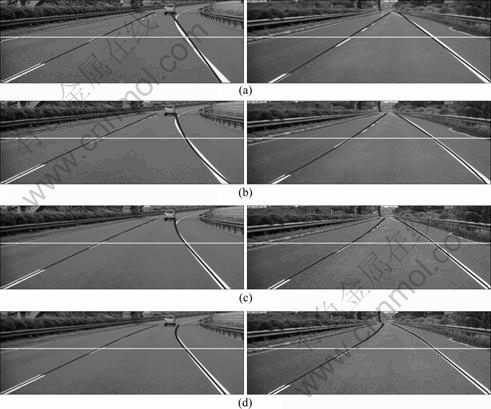
Fig. 4 Comparison of several road models (White horizontal line is division between near region and far region): (a) Straight line model; (b) Parabola model; (c) Linear-parabolic model; (d) Linear-cubic model

Table 1 Results from standard deviations of fitting errors of right boundary lines in Fig. 4 (Unit: Pixel)

In this work, a novel general object feature, named feature line section (FLS), is proposed for lane marking detection by combining multiple low-level features and the uniqueness of the target object. Defined in the image coordinate system, FLS is a kind of specific horizontal line sections in images. An FLS is normally represented as FLS(u_L, u_R, v), where u_L denotes the horizontal ordinate of the left terminal point of FLS, u_R denotes the horizontal ordinate of the right terminal point of FLS and v represents the vertical ordinate of FLS, which must satisfy the following three constraints:

1) Appearance constraint (AC): The intensity of all points contained in an FLS, denoted by P(x, v)(x∈[u_L, u_R], is a stochastic variable with a certain probability distribution according to the object appearance.

2) Edge constraint (EC): The two terminal points of FLS, P(x_L, v) and P(x_R, v) must satisfy some edge constraints according to the object contour.

3) Width constraint (WC): The width of FLS, i.e., (u_R-u_L), must meet some inequality restrictions according to the object real width.

The above three constraints are described in a general form. When the target object is determined, the constraints will be defined in detail according to the features of the target object. The definition of the constraints should be easy to be verified. If a constraint is hard to be verified directly, an indirect form of the constraint can be used for verification. For example, if the probability distribution in AC is hard to be verified, some simple statistical quantities of all points contained in an FLS can be used to verify whether the constraint is satisfied or not, such as the average value of the intensity.

It should be noticed that the lane markings are brighter than the road regions. They also have clear edges. Furthermore, the width of the lane markings, which usually is about 10 cm, is always fixed. This observation means that there is a constraint in the width of lane markings. Therefore, the constraints on FLS(u_L, u_R, v) for lane marking detection are easy to be defined as follows:

                     (2)

               (3)

                    (4)

Inequation (2) means that the mean of the pixels in the FLS must be greater than a threshold value P_T. The threshold value P_T can be obtained by an adaptive approach similar to the approach proposed in Ref. [21]. Inequation (3) means that the two terminal points of the FLS must be horizontal edges. The parameter S_T is a fixed edge threshold value determined by experiences. It is set to be 15 in practice. The horizontal Sobel operator E_HS(u, v) is used for computing horizontal edge values. Inequation (4) represents the width constraint. The threshold values L_L(v) and L_H(v) can be computed by camera calibration parameters and the actual width of the vehicle with the assumption of flat roads. The horizontal line sections on the lane markings in Fig. 5 are examples of FLSs for lane marking detection. It can be noticed that the tiny lane markings in far regions can still be extracted as FLS.

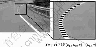
Fig. 5 FLS for lane marking detection

The comparison among white color region detection, edge detection with the Sobel operator and the FLS extraction is shown in Fig. 6. The threshold value used in white color region detection is the same parameter P_T, and the threshold value used in edge detection is also S_T. It is easy to see that over 80% extracted FLSs exist in lane marking regions while less than 50% pixels extracted by white color region detection and edge detection are in lane marking regions. The conclusion is obvious that the FLS extraction, which can effectively avoid the undesired influences of large bright areas and disordered edges in the background, is more accurate and more efficient for lane marking detection.

3.2 Fast FLS extraction

In practice, many feature extraction methods usually cost a lot of time. For meeting the real-time requirement of autonomous vehicles, a fast FLS extraction algorithm is presented for lane detection. Obviously, the efficiency of this algorithm depends on the constraints of an FLS.  If the constraints are not complex, the FLS extraction

algorithm can be computationally efficient. Based on the three constraints introduced in the previous sub-section, the fast FLS extraction algorithm can be designed for lane marking detection. The main steps of the fast FLS extraction algorithm are described in Algorithm 1. The results of FLS extraction are shown in Fig. 7(b).

Algorithm 1 Fast FLS extraction algorithm

Initialization:

Input image G. Result set FLS=f. Edge point set LE=RE=f.

Extraction:

1) Scan all points P(u, v) in line v of G. P(u, v)∈LE if HSobe(u, v)<-S_T; P(u, v)∈RE if HSobe(u, v)T.

2) Get out a point X(u, v)∈LE. Then, check all points in RE one by one. If find a point Y(u_y, v)∈RE to let line section LS(u_x, u_y, v) satisfy Eqs. (2) and (4), LS(u_x, u_y, v)∈FLS and cancel out all u≤u_y points in LE.

3) Repeat Step 2, until LE=f.

4) Repeat Steps 1-3, until all lines of G have been processed.

3.3 Lane line generation

3.3.1 Clustering FLS features

After all the FLS features are extracted from the input image, they should be clustered by using appropriate clustering algorithms. Since the number of lane markings in the input image, i.e., the number of clusters, is unknown, the classic nearest neighbor (NN) clustering algorithm is chosen to process all the FLS features in this work. Another reason for this choice is that the computational cost of the nearest neighbor clustering algorithm is extremely low without any iterative process, which is very beneficial for developing a real-time algorithm. The difference between a normal NN clustering algorithm and the algorithm used in this work is that each cluster is forced to contain at most only one FLS in a line of the input image. This constraint makes the FLS of two lane lines divided into two clusters even if the distance of the two lines is very short (see  Fig. 8). Finally, the clusters only containing very few FLSs will be deleted. The clustering result is shown in Fig. 7(c).

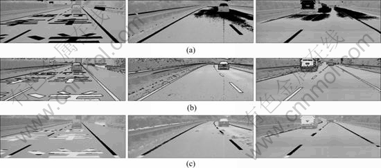
Fig. 6 Comparison among results of different feature detection (Black pixels are results of detections): (a) White color region detection; (b) Edge detection; (c) FLS extraction

 

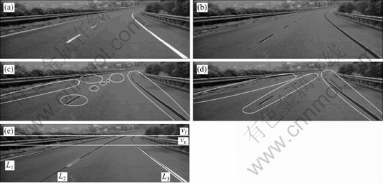
Fig. 7 FLS extraction and lane line generation: (a) Original image; (b) FLS extraction; (c) Clustering FLS; (d) Connecting clusters; (e) Fitting road model

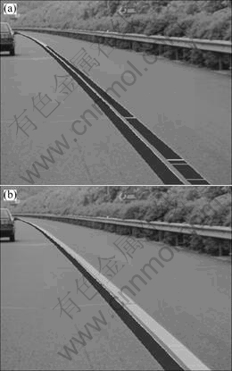
Fig. 8 Results of nearest neighbor clustering algorithms: (a) One cluster (black) without FLS/one line constraint; (b) Two clusters (black and grey) by using constraint

3.3.2 Connecting clusters

It can be noticed that a lane line, especially the middle segmented line, is composed of several clusters. These clusters should be connected into a lane line. Assuming that a cluster can be approximated by a line section, the connecting method is to compute the scope rate of every cluster by putting the center points of all FLSs into a least-squares fitting process. Then, the scope rates are compared. Finally, two clusters with similar scope rates and a short distance between the first FLS of one cluster and the last FLS of the other cluster are connected as one cluster. The result of connecting clusters is shown in Fig. 7(d).

3.3.3 Fitting road model

After connecting clusters, the short clusters are deleted imperatively. The rest clusters are used to fit the road model. A cluster fits a lane line. The fitting method used in this work is least-square fitting. Firstly, the center points of the FLSs in the near region (u_i, v_i)(i∈[1, k]) are used to fit a straight line and the parameters α and β are obtained as follows:

(5)

  (6)

Secondly, the center points of FLSs in the far region (u_i, v_i)(i∈[k+1, m]) are used to compute the parameter γ and λ as follows:

 (7)

 (8)

Finally, several lane lines L_x (x=1, 2, …, n) are obtained. The result of road fitting is shown in Fig. 7(e).

4 Lane tracking

4.1 Lateral offset and heading angle

After obtaining the parameters of the road model, the lateral offset and heading angle of an autonomous vehicle can be estimated by each lane line. Lateral offset and heading angle are two important states of an autonomous vehicle. They are used in many integrated functions, such as adaptive lane keeping, automatic vehicle control and autonomous lane-change. They will also be used to track the lanes in this work. Furthermore, the number of detected lane lines may be more than three. Correct lines should be picked out from them in tracking according to lateral offsets and heading angles too. The autonomous vehicle is called as the ego vehicle in the following discussions.

Before estimating the lateral offset and heading angle of an autonomous vehicle, all the lane lines obtained in the lane detection process, which are denoted as L_x (x=1, 2, …, n), must be classified as solid lines or segmented lines. A saturation degree function f(L_x) is defined as follows:

             (9)

where N(L_x) means the number of FLSs contained in L_x, V_max(L_x) and V_max(L_x) denote the maximum v and the minimum v of all FLS(u_x, u_y, v) contained in L_x, respectively.

Then, a simple classifier is defined as follows:

                      (10)

where S is the set of the solid lines and G is the set of the segmented lines.

Before estimating the lateral offset O_x and heading angle θ_x of the autonomous vehicle, two points are chosen in the near region at first and they are denoted as (u₁, y₁)∈L_x(v₁≥v_n) and (u₂, y₂)∈L_x(v₂≥v_n). Then, the corresponding points in the world coordinate system, (x₁, y₁) and (x₂, y₂), can be computed using camera calibration data and the assumption of flat roads (see  Fig. 9). Finally, the heading angle of the autonomous vehicle can be estimated using Eq. (11) and the lateral offset can be estimated using Eq. (12) as follows:

                 (11)

         (12)

where

                          (13)

                          (14)

where W_lane means the width of the lane, which is usually fixed on highway roads. Assuming that the autonomous vehicle is always on the road, a solid lane line is classified as a left boundary line if C_x<0; otherwise, it is classified as a right boundary line. All segmented lines are considered as middle lines.

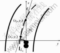
Fig. 9 World coordinate system and ego vehicle lateral offset

4.2 Lane lines selection and tracking

It is possible that more than one left boundary lines/right boundary lines/middle lines are generated in an input image. They are selected by a lane tracking algorithm. The lane lines are tracked by estimating the ego vehicle lateral offset and heading angle with a Kalman filter. The difference between the filter used in this work and a normal filter is that a lane line selection process is inserted between the prediction process and the update process of the filter. The selection process is performed according to the predicted ego vehicle lateral offset and heading angle. Then, the lateral offset and heading angle of ego vehicle are used in the update process. The flow chart of the lane tracking algorithm is shown in Fig. 10.

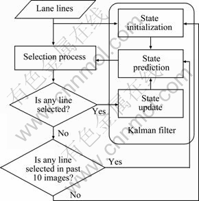
Fig. 10 Flow chart of lane tracking algorithm

At time k, the change rates of the ego vehicle lateral offset O(k) and heading angle θ(k) are ?O(k) and ?θ(k), respectively. For simplicity, the heading angle θ(k) can be considered to change in a constant rate. Because θ(k) is usually very small in practice, the state vector x=[θ(k) ?θ(k) O(k) ?O(k)]′ of ego vehicle is predicted as follows:

    (15)

The lane lines are selected using  and  Since a heading angle value and a lateral offset value can be computed by a detected lane line, the predicted heading angle  and the predicted lateral offset  can be considered as the reference for selecting the correct lane line. For example, if multiple right boundary lines L_x (x=1, 2, …, n) are generated, the line L_r with heading angle θ_r and lateral offset O_r is selected as the right boundary line only if the following function F(x) is minimized when x=r:

       (16)

where α and β are adjustable weight values in this implementation. In practice, they are set as α=10 and β=1.

Moreover, the line L_r must satisfy

 and            (17)

where D_T is the threshold of the differences between the predicted heading angle and the detected heading angle, and E_T is the threshold of the differences between the predicted lateral offset and the detected lateral offset. They can be set as D_T=0.1 and E_T=0.5 m in practice.

Similarly, θ_m, O_m, θ_l and O_l can be obtained as above if one or more middle lines and left boundary lines are generated. Then, the measurement vector  is computed as follows:

                      (18)

where  and  and the subscript d is one element of the set {l, m, r}. When x=d, the function F(x) (x∈{l, m, r}) defined in Ref. (16) is minimized.

Using the lateral offset and heading angle of ego vehicle, the correct lane lines can be selected with an extremely high probability even if the distance between the correct line and the wrong line is very short. Figure 11 shows some results of lane line selection and tracking in real traffic scenes. It can be seen that the proposed lane detection and tracking approach still work well in various challenging scenarios. The results of the experiment with more than 3 000 saved road images show that the approach can achieve an average correct detection rate of 94.37% with an average false positive detection rate of 0.35%, contrary to an average correct detection rate of 90.8% reported in Ref. [16]. The tracking process extremely decreases the false positive detection rate.

Running on a current PC based on AMD Athlon64 3000+, the average time cost of the proposed lane detection and tracking approach is low at 12.9 ms per frame. The performance of the approach is undoubtedly real-time.

5 Front vehicle location

One of main aims of long-distance lane perception is front vehicle location. Front vehicle location is very important for driving strategy and action selection of full autonomous vehicles. If the front vehicle is in a different lane, the autonomous vehicle can keep its speed without considering the speed of the front vehicle. If the front vehicle is on the same lane as the ego vehicle, the autonomous vehicle must decide to keep the distance or to change its lane and overtake it. However, this topic is rarely explored in previous researches.

Since the extrinsic camera parameters may change due to vehicle pitch and the assumption of flat roads is not satisfied in many cases, large errors may occur when computing the lane position in the world reference system using the extrinsic camera parameters and the assumption of flat roads. Considering these errors and the errors caused by the information delay described in Ref. [22], it is appropriate that front vehicle location is performed in image field. Therefore, the exact positions of lane lines and front vehicles in input images are needed. The exact positions of lane lines can be obtained by the algorithm described in the above sections while the exact positions of front vehicles can be detected by a vision-based vehicle detection algorithm presented in Ref. [23].

There are five states of a front vehicle: left lane, right lane, out of left lane, out of right lane and crossing the middle line. A state set {L, R, O_L, O_R, M} is built for location. The exact position of a front vehicle is often represented as a bounding box V_Box(u_VL, u_VR, v_T, v_B). The exact positions of lane lines are represented as u_x=f_x(v) (x∈{L, M, R}) according to Eq. (1). The front vehicle state classifier is easy to be defined as follows:

     (19)

If a lane line is not detected, some judgments in Eq. (19) cannot be completed. In these cases, the distance between the front vehicle and the detected lane line is computed to locate the front vehicle on the correct lane instead. For example, if the right boundary line is not detected, f_R(v_B) cannot be obtained. The distances in

world coordinates between the left bottom corner of the front vehicle p(u_VL, v_b) and the corresponding point of the middle line p(f_M(v_B), v_b) can be computed as follows:

   (20)

where  is the transfer function from the image coordinates to the world coordinates. It is defined by the camera calibration parameters with the assumption of flat roads. Then, the state classifier for front vehicles is changed as follows:

   (21)

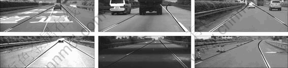
Fig. 11 Some results of lane line selection and tracking (Black lines are correct while white lines are wrong lane lines)

If the left boundary line is not detected, the classifier is similar to Eq. (21). But if the middle line is not detected, the classifier should be changed as

      (22)

where

    (23)

   (24)

If only one lane line is detected, more judgments in the classifier are performed by using the distance between the front vehicle and the detected lane line. Since the distance is computed by camera calibration parameters with the assumption of flat roads, it usually contains large errors. Therefore, a great number of false locations appear when only one lane line is detected. In a word, the more the lane lines are detected, the more possible the front vehicle is to be located on the correct lane. Figure 12 shows some results of front vehicle location in real traffic scenes. It can be noticed that the maximal location distance is more than 120 m.

6 Experiments

6.1 HQ3 full autonomous vehicle

The HQ3 full autonomous vehicle (HQ3-FAV) is a full autonomous vehicle running on highway roads refitted from a FAW HQ430 Sedan (see Fig. 13). HQ3-FAV has many integrated functions of adaptive lane keeping, autonomous lane-change, overtaking, and traffic flow joining. The main components of HQ3-FAV include:

1) Road environment perception system (REPS);

2) Driving strategy and action selection system;

3) Automatic vehicle control system;

4) Controller-area-network (CAN) interface for acquiring wheel velocities, steering angle and other vehicle information.

The sensors of the REPS include:

1) Two forward-looking IEEE 1394 cameras and one back-looking IEEE 1394 camera;

2) One forward-looking 76GHz MMW radar and one back-looking 76GHz MMW radar;

3) Two lateral-looking single-beam laser radars.

For meeting the requirements of long-distance lane perception and front vehicle location, a forward-looking IEEE 1394 monocular camera with a 1 024×384 resolution and a 16 mm focus length shown in Fig. 13 is used for lane detection, tracking and front vehicle location. The camera has a horizontal opening angle of about 25° and a maximal update rate of 15 Hz. The final update rate of lane detection, tracking and front vehicle location module is 10 Hz. The maximal lane detection and tracking distance is up to 120 m by using the algorithm presented in this work. Likewise, the maximal effective distance of front vehicle location is also 120 m.

6.2 Long-distance full autonomous drive experiment

A 286 km full autonomous drive experiment has been conducted successfully by HQ3-FAV under real traffic conditions on July 14th, 2011. The route of this experiment is from Changsha to Wuhan, following G4 Jing-Gang-Ao Highway Road (see Fig. 14).

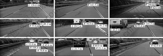
Fig. 12 Some results of front vehicle location

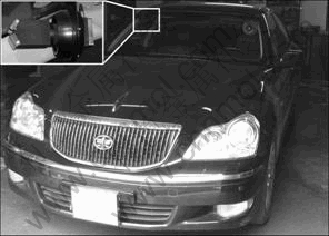
Fig. 13 HQ3 full autonomous vehicle and camera used for lane detection and tracking

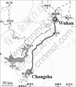
Fig. 14 Route of long-distance full autonomous drive experiment

The percentage of full autonomous drive in distances was high at 99.22%. HQ3-FAV spent 3 h and 22 min to complete this trip by driving itself autonomously. The actual average speed of HQ3-FAV in this experiment was about 85 km/h, which was lower than the cruise speed of 100 km/h. It was entirely the result of heavy traffic. During the experiment, there were a great number of slow heavy trucks on G4 Highway Road. They often occupied both lanes, which had forced HQ3-FAV to follow them at low speed for a long time.

In this experiment, the steer, throttle, brake, tune lights and speakers of HQ3-FAV were all controlled by computers. It still ran in autonomous mode safely even if it met various complex road environments and bad weather including: 1) extremely heavy traffic, 2) poor lane markings, 3) heavy rain and 4) light fog.

In this experiment, hundreds of difficult actions, including autonomous lane-change, autonomous overtaking, and being overtaken by other vehicle, were performed successfully by HQ3-FAV. Moreover, HQ3-FAV joined in high-speed traffic flow autonomously more than 10 times. When heavy rain fell down, HQ3-FAV still changed its lane and overtook heavy trucks safely (see Fig. 15). The experimental data, including total distance of the experiment, percentage of full autonomous drive in distance, number of autonomous lane-changes, number of autonomous overtaking, number of being overtaken by other vehicles, number of traffic flow joining and number of human intervention, are listed in Table 2.

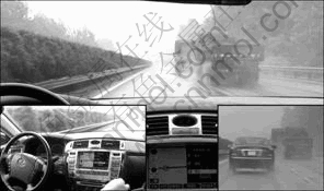
Fig. 15 HQ3-FAV overtaking heavy trucks in heavy rain

6.3 Evaluation of lane detection, tracking and front vehicle location

The most common metrics for lane detection and tracking performance evaluation include mean absolute error in lateral offset, standard deviation of error in lateral offsets, and standard deviation of errors in changing rate of lateral offsets [5], etc. However, the quantitative results of the evaluation in the long-distance full autonomous driving experiment cannot be provided for the lack of ground truth data for lateral offsets. Here, an ego vehicle state dataset, including lateral offsets, changing rates of lateral offsets, heading angles and changing rates of heading angles, is shown in Fig. 16 for the performance evaluation of the proposed lane detection and tracking approach. The dataset shows two lane-change processes of HQ3-FAV obviously.

Table 2 Experimental data

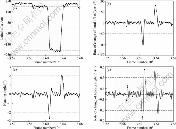
Fig. 16 Ego vehicle state dataset: (a) Lateral offset; (b) Rate of change of lateral offset; (c) Heading angle; (d) Rate of change of heading angle

The qualitative evaluation for the proposed lane detection and tracking approach can be obtained by the experimental data shown in Table 2. Long-distance lane keeping and hundreds of lane-change were successfully executed by HQ3-FAV according to the lane information obtained by the proposed lane detection and tracking approach. Even if in heavy rain and light fog, the lane information extraction was not interrupted. Furthermore, none of the human interventions was caused by false results of lane detection and tracking. All of these results indicate that the proposed lane detection and tracking approach is effective and robust enough for full autonomous drive.

In this experiment, the proposed front vehicle location approach has been performed more than    100 000 times. The quantitative results of the evaluation cannot be provided for the lack of ground truth data. However, hundreds of autonomous overtaking actions were correctly promoted in time by the driving strategy and action selection system while no false lane-change decision was made in response to the faults of front vehicle location. This result means that the proposed front vehicle location approach achieves a high correct rate of location.

The time cost of the proposed lane detection, tracking and front vehicle location approaches is very low. Running on a current PC based on Intel T2390 CPU with saved images, the update rate of the approaches is high at more than 50 Hz. It is to cooperate with other modules of the REPS that the lane detection, tracking and front vehicle location module runs at a low update rate of 10 Hz.

7 Conclusions

1) Due to large fitting errors of many road models in far regions, a linear-cubic road model with small fitting errors both in near and far regions is presented for long-distance lane detection.

2) Combining the constraints of intensity, edge and width, FLS, a novel robust lane marking feature is presented for lane marking extraction. Owing to the usage of prior knowledge in FLS definition, the lane marking extraction algorithm can extract the tiny lane markings in far regions accurately and efficiently, while it can avoid the undesired influences of large bright areas and disordered edges in backgrounds.

3) The lane tracking approach is based on the estimation of the lateral offset and heading angle of ego vehicle with a Kalman filter. Since the lateral offset and heading angle can be computed by each lane line, the predicted lateral offset and heading angle are used as the reference for lane line selection in the tracking process. It is a relaxed lane tracking approach that requires correct positions and angles of the lane lines in near regions only. Using this approach, the tracked lane lines will not be missed even if some parts of the lane lines in far regions have changed quickly.

4) Front vehicle location is performed in image coordinates rather than world coordinates. It has a higher correct rate of vehicle location because large errors may occur when computing the lane position in world coordinates, especially in far regions.

References

[1] Amditis A, Bertolazzi E, Bimpas M, Biral F, Bosetti P, Lio D M, Danielsson L, Gallione A, Lind H, Saroldi A, Sjogren A. A holistic approach to the integration of safety applications: The INSAFES subproject within the European framework programme 6 integrating project PReVENT [J]. IEEE Transactions on Intelligent Transportation Systems, 2010, 11(3): 554-566.

[2] Amditis A, Bimpas M, Thomaidis G, Tsogas M, Netto M, Mammar S, Beutner A, Mohler N, Wirthgen T, Zipser S, Etemad A, Lio D M, Cicilloni R. A situation-adaptive lane-keeping support system: Overview of the SAFELANE approach [J]. IEEE Transactions on Intelligent Transportation Systems, 2010, 11(3): 617-629.

[3] Kwon W, Lee S. Performance evaluation of decision making strategies for an embedded lane departure warning system [J]. Journal of Robotic Systems, 2002, 19(10): 499-509.

[4] Lee J W, Kee C D, YI U K, A new approach for lane departure identification [C]// Proceedings of IEEE Intelligent Vehicles Symposium. Columbus, OH, 2003: 100-105.

[5] McCall J C, Trivedi M M. Video-based lane estimation and tracking for driver assistance: survey, system, and evaluation [J]. IEEE Transactions on Intelligent Transportation Systems, 2006, 7(1): 20-37.

[6] McCall J C, Trivedi M M. Visual context capture and analysis for driver attention monitoring [C]// Proceedings of IEEE Conference on Intelligent Transportation Systems. Washington D C, 2004: 332-337.

[7] Salvucci D D. Inferring driver intent: A case study in lane-change detection [C]// Proceedings of Human Factors Ergonomics Society 48th Annual Meeting. New Orleans, LA, 2004: 2228-2231.

[8] Bertozzi M, Broggi A. GOLD: A parallel real-time stereo vision system for generic obstacle and lane detection [J]. IEEE Transactions on Image Process, 1998, 7(1): 62-81.

[9] Eidehall A, Gustafsson F. Obtaining reference road geometry parameters from recorded sensor data [C]// Proceedings of IEEE Intelligent Vehicles Symposium. Tokyo, Japan, 2006: 256-260.

[10] Wang Yue, TEOH E K, Shen Ding-gang. Lane detection and tracking using B-Snake [J]. Image Vision Computing, 2004, 22(4): 269-280.

[11] CHEN Qiang, WANG Hong. A real-time lane detection algorithm based on a hyperbola-pair model [C]// Proceedings of IEEE Intelligent Vehicles Symposium. Tokyo, Japan, 2006: 510-515.

[12] Hendrik W, Philipp L, Gerd W. Vehicle tracking with lane assignment by camera and lidar sensor fusion [C]// Proceedings of IEEE Intelligent Vehicles Symposium. Xi’an, China, 2009: 513-520.

[13] Simond N. Reconstruction of the road plane with an embedded stereorig in urban environments [C]// Proceedings of IEEE Intelligent Vehicles Symposium. Tokyo, Japan, 2006: 70-75.

[14] He Ying-hua, Wang Hong, Zhang Bo. Color-based road detection in urban traffic scenes [J]. IEEE Transactions on Intelligent Transportation Systems, 2004, 5(4): 309-318.

[15] RASMUSSEN C. Texture-based vanishing point voting for road shape estimation [C]// Proceedings of British Machine Vision Conference. Kingston, UK, 2004: 470-477.

[16] WANG Yan, BAI Li, FAIRHURST M. Robust road modeling and tracking using condensation [J]. IEEE Transactions on Intelligent Transportation Systems, 2008, 9(4): 570-579.

[17] Jung R, Kelber C R. A robust linear-parabolic model for lane following [C]// Proceedings of Brazilian Symposium on Computer Graphics and Image. Sao Leopoldo, Brazil, 2004: 72-79.

[18] KIM Z. Robust lane detection and tracking in challenging scenarios [J]. IEEE Transactions on Intelligent Transportation Systems, 2008, 9(1): 16-26.

[19] LIU Xin, SUN Zhen-ping, HE Han-gen. On-road vehicle detection fusing radar and vision [C]// Proceedings of IEEE International Conference on Vehicular Electronics and Safety. Beijing, China, 2011: 150-154.

[20] Liu Feng, Sparbert J, Stiller C. IMMPDA vehicle tracking system using asynchronous sensor fusion of radar and vision [C]// Proceedings of IEEE Intelligent Vehicles Symposium. Eindhoven, Netherlands, 2008: 168-173.

[21] Tzomakas C, Seelen W. Vehicle detection in traffic scenes using shadows [R]. Bochum, Germany: Institut fur Neuroinformatik, Ruht-Universitat, 1998.

[22] XIAO Ling-yun, GAO Feng. Effect of information delay on string stability of platoon of automated vehicles under typical information frameworks [J]. Journal of Central South University of Technology, 2010, 17(6): 1271-1278.

[23] LIU Xin, DAI Bin, HE Han-gen. Real-time on-road vehicle detection combining specific shadow segmentation and SVM classification [C]// Proceedings of International Conference on Digital Manufacturing and Automation. Zhangjiajie, China, 2011: 885-888.

(Edited by YANG Bing)

Foundation item: Project(90820302) supported by the National Natural Science Foundation of China

Received date: 2011-06-31; Accepted date: 2011-10-13

Corresponding author: LIU Xin, PhD; Tel: +86-731-84576145; E-mail: liuxin@nudt.edu.cn