J. Cent. South Univ. (2018) 25: 936-948

DOI: https://doi.org/10.1007/s11771-018-3795-7

Method for secondary spring load equalization of railway vehicles with two-stage spring suspension: Modeling and optimal regulation

BAO Tian-zhe(鲍天哲)^{1, 2}, HAN Kun(韩锟)¹, PAN Di-fu(潘迪夫)¹

1. School of Traffic and Transportation Engineering, Central South University, Changsha 410075, China;

2. School of Electronic and Electrical Engineering, University of Leeds, Leeds, UK

Central South University Press and Springer-Verlag GmbH Germany, part of Springer Nature 2018

Abstract: To ensure running safety, the secondary spring loads of railway vehicles must be well equalized. Due to the coupling interactive effects of these hyper static suspended structures, the equalization adjustment through shimming procedure is quite complex. Therefore, an effective and reliable method in application is developed in this paper. Firstly, the best regulation of spring load is solved based on a mechanical model of the secondary suspension system, providing a target for actual adjustment. To reveal the relationship between secondary spring load distribution and shim quantity sequence, a forecasting model is constructed and then modified experimentally with consideration of car body’s elastic deformation. Further, a gradient-based algorithm with a momentum operation is proposed for the load optimization. Effectiveness of the whole method has been verified on a test rig. It is experimentally confirmed that this research provides an important basis for achieving an optimal regulation of spring load distribution for multiple types of railway vehicles.

Key words: railway vehicle; secondary spring load equalization; optimal regulation; shimming procedure; elastic deformation

Cite this article as: BAO Tian-zhe, HAN Kun, PAN Di-fu. Method for secondary spring load equalization of railway vehicles with two-stage spring suspension: Modeling and optimal regulation [J]. Journal of Central South University, 2018, 25(4): 936–948. DOI: https://doi.org/10.1007/s11771-018-3795-7.

1 Introduction

The body and axles of a railway vehicle with two-stage suspension are supported by four or more primary and secondary springs, respectively. Owing to the great mass of the body and the high stiffness of springs, even small manufacturing errors, load-dependent deformations and changes in the features of spring elements (elasticity and geometric dimensions) will cause different load on the spring supporting points, and eventually result in substantial different loads of wheels on the track. However, it is required that the total weight of each unit in a railway vehicle should be distributed substantially equally on all of its wheels when weighed at rest since the wheel load distribution of railway vehicles has been a critical factor influencing the safety, efficiency, and reliability of railway transport [1]. Considering expected further increases in the running speed of railway vehicles, the permissible deviations of static wheel loads are specified in many national and international standards or criteria [2–4].

In this case, a special shimming procedure has been adopted in the assembling process as a crucial means to control the load distribution. If the load distribution is not as desired, it is adjusted by adding shims to the seats of the primary and secondary springs selectively. Since the distribution of secondary spring loads plays a more significant role for equalization of wheel loads after assembly, many railway vehicle companies in China have drawn up their own criteria for this adjustment through shimming procedure. However, this complex load redistribution process is full of multi-factors coupling interactive effects. Any increment in weight caused by an added shim at one spring seat must of course result in a net weight decrement of equal amount at other springs, since the two-stage spring suspension system is statically indeterminate and the total weight of the vehicle is constant. In traditional way, the adjustment process is conducted by trial and error, which is relied heavily on sense and experience of the operators. This would be very inefficient, inexact and costly, which cannot adapt to the requirement of modern manufacturing. So, a new accurate and reliable method becomes a necessity.

Up to now, many scholars have studied the regulation process of railway vehicles’ spring system by using empirical, experimental and analytical methods. BELOBAEV [5] once put forward an empirical formula to determine the sizes of shims required at designated axles. CURTIS et al [6] pioneered the study on the method of adjusting the distribution of locomotive axle loads in USA by presenting experimental solutions. RUZHEKOV et al [7] analyzed the effect of locomotive spring system parameters on the static wheel load distribution, and then they developed a mathematical model [8] of the railway vehicle spring suspension to reveal dependencies determining the condition of the best regulation. TANAKA [9] used a calculation method to forecast the static wheel load, and also investigated the influence of eccentric vehicle C.G. on the static wheel load. HAN et al [10] employed the axle weight transfer model and extended it to calculate the additional axle load caused by adding shims. All of these studies provided useful guidelines for the optimal adjustment of wheel load distribution, and most of them have been applied in some automatic load management device for railway vehicles [11–13]. As is reported obviously, this kind of adjustment is quite complex. Many problems, such as what is the relationship between shim sizes and load distribution, what is the optimal state of load distribution, what is the condition of the best regulation, are still not clear for lack of deep analysis in theory.

The work here is devoted to the analysis and achievement of secondary spring load equalization based on statistics, modeling and engineering practice, aiming to propose an efficient and reliable method for optimal regulation through shimming procedure. Here the secondary suspension works as the research object for three main reasons. Firstly, the static wheel load deviation caused by poor secondary spring load distribution cannot be ameliorated through adjustment on the primary suspension. Secondly, the spring load regulation is more difficult for secondary suspension, since it has a higher degree of indeterminacy statically and a greater nonlinearity due to the car body’s elastic deformation. Furthermore, the car body becomes more interchangeable in application after corresponding adjustment.

The remainder of this paper is divided as follows: in Section 2 we focus on the problem statement of the main research. In Section 3 the best regulation state of spring load distribution with distinguish conditions has been investigated in detail, aiming to give a guidance for the adjustment. Section 4 establishes the secondary spring load forecasting model, so that we could have a clearer perspective of the relationship between secondary spring load distribution and the shim quantity sequence. To improve the accuracy of this model further, an effective modification in consideration of the car body’s elastic deformation is proposed. Section 5 studies the optimal method for the equalization which could be solved by a gradient- based algorithm efficiently. Based on these above, the whole method is constructed eventually to guide the shimming procedure. Modification of the forecasting model is done and verified experimentally in Section 6.1. Section 6.2 together with Section 6.3 shows the effectiveness of this method on multiple types of railway vehicles.

2 Problem statement

To best illustrate the modeling and regulation method, we base our discussions on a locomotive of the C0–C0 axle arrangement. The structural illustration of the locomotive suspension system is shown in Figure 1.

Figure 1 Structural illustration of C0–C0 suspension system

The secondary suspension system of the locomotive is considered here. It consists mainly of the body and the secondary springs, as shown in Figure 1. The aim of the secondary spring regulation is to compensate the change of the features of the secondary spring elements and possibly disturbed geometry, weight and elasticity of the body, and to minimize the existing differences among the secondary spring loads. When all those reasons are removed, it is called “the best regulation”.

The shimming procedure is conducted in a test rig wherein four groups of movable weighing stands with three per group are lowered in the same horizontal plane, as shown in Figure 2. Each weighing stand includes a load cell for measuring the actual weight of any heavy object placed on top of it and a hydrostatic actuator adjustable in height for adjusting lower surface of the secondary spring to simulate the added shims.

Figure 2 Test rig for regulation of locomotive secondary spring load distribution

To achieve a substantially equal or balanced secondary spring load distribution, the whole solution can be obtained as follows.

1) Measure the load that is impressed on each weighing stand after the locomotive body and secondary springs are in place on the test rig.

2) Build a model to obtain the optimal distribution of secondary spring load and work out the dependencies and criterions determining the condition of the best regulation.

3) Use the criterions to judge if the best regulation is achieved.

4) If the load distribution is not as desired, conduct adjustment quality calculation to predict the particular combination and sizes of shims that are required to obtain a substantially equal distribution of load on all secondary springs. To determine the optimal shim quantity sequence, a secondary spring load forecasting model is established and optimized by experimental data firstly. The optimal shim quantity sequence is then given based on the forecasting model using a gradient-based algorithm with adapted step.

5) Raise the actuators to simulate the indicated shims and measure the new load, and then repeat steps 3)–5) until the best regulation is achieved.

The framework of the whole method is demonstrated in Figure 3.

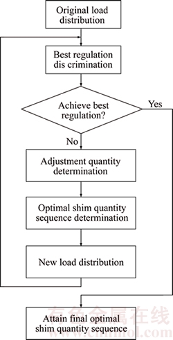
Figure 3 Flow diagram of whole method

As mentioned before, the considered system is statically indeterminable. This makes the law of spring load distribution more complex. So, we restrict ourselves to the following class of systems and system models:

1) Only vertical loads are considered;

2) Deformations of locomotive body and influence of the height of body’s barycenter are ignored. So the body is considered to be a plane rigid frame;

3) Locomotive secondary suspension system is considered symmetric and the lower surfaces of all secondary springs are assumed to be in the same horizontal plane. This plane is considered to be the base of the model;

4) Parallel springs on the same side of a bogie are regarded as a single spring on the basis of some equivalent criteria.

Based on the assumptions mentioned above, the simplified geometry model of the considered system is expressed in Figure 4. The coordinate frame O-XYZ is fixed on the geometric center of the base plane, and the O-X axle is parallel to longitudinal direction of the body. F₁, F₂, F₃ and F₄ are support forces at various points loaded by the secondary springs. G is the gravity force of the body. e_x and e_y are coordinates of the projection of the body mass center on the base plane. a and b are the geometric parameters of the body.

Figure 4 Simplified geometry model of secondary suspension system

3 Analysis of best regulation conditions

As described above, it is significant to understand the state of the best regulation and work out the related criterions. Otherwise, there can be no assurance that an adjustment is optimal in the sense of minimum-variance. In this study, a quadratic programming model is built to solve the problem.

3.1 Conditions for best regulation

In Figure 4, there are four support forces F₁, F₂, F₃ and F₄ which act on the car body. The ideal distribution of them should be as follows:

                      (1)

In practice, the actual forces F-designations are deviated from the ideal values for many reasons. The mean square error (MSE) of them could be applied to reflecting the uniformity of load distribution. Obviously, the smaller the MSE is, the more uniform the force distribution will be.

So the mean square error of the forces is taken to be the optimization objectives, which can be expressed as:

                        (2)

where F₁, F₂, F₃ and F₄ are decision variables and J is the objective.

Based on the forces loaded on the body described in Figure 3, the static equilibrium equation of the body is established. It can be given as:

                 (3)

Thus, the quadratic programming model of best regulation state is given by

              (4)

Solving this quadratic programming model by direct elimination method, the optimal solution set of load distribution F₁^*, F₂^*, F₃^* and F₄^* can be obtained by

                      (5)

Therefore, the minimum MSE of four support forces is obtained when F₁, F₂, F₃ and F₄ are equal to F₁^*, F₂^*, F₃^* and F₄^* respectively. Equation (5) is the sufficient condition for that the secondary spring load distribution is optimal and the best regulation can be determined by it.From Eq. (5), we have

                         (6)

The physical meaning of Eq. (6) can be explained as follows: sums of the forces at the body’s opposite ends are the same when secondary spring load distribution reached its optimization and the best regulation is achieved. Equation (6) is the necessary condition of the best regulation. That is, it is impossible to achieve the best regulation unless F₁, F₂, F₃ and F₄ satisfy Eq. (6).

Based on the above analysis, Eq.(6) can be used to identify most non-optimal regulations.

Equation (6) seems to work for this purpose in theory. However, in practice, the sum of the forces at one diagonal could not exactly equal to the other due to the measurement errors. This may lead to an infinite loop. Therefore, an improved criterion derived from Eq. (6) is presented to do the pre-judgment. It is given by

                     (7)

where δ is a very small positive quantity.

3.2 Method of best regulation discrimination

The steps of the proposed method are described as follows:

1) Measure the load that is impressed on each weighing stand and do aggregate calculation to attain the corner forces, F₁, F₂, F₃ and F₄.

2) Make pre-judgment by using Eq. (7). The judgment rules are: If F₁, F₂, F₃ and F₄ do not satisfy Eq. (7), it can be concluded that the best regulation is not reached and further adjustment is needed. Otherwise, the best regulation is reached and the adjustment can be stopped.

4 Secondary spring load forecasting model

Section 3.2 draws a blue print for the adjustment of secondary spring load distribution, but there still remains a key problem on how to achieve this goal through the shimming procedure. As mentioned before, the relationship between shim sizes and deviations from desired weight distribution is statically indeterminate, so it is a critical issue to select suitable sizes of shims to add at proper load points to equalize the static distribution of the total locomotive body weight on the respective secondary springs.

In this case, a secondary spring load forecasting model should be established to reveal the relationship between secondary spring load distribution and the shim quantity sequence, so that we could have a better perspective of the change laws.

4.1 Model establishment

According to the geometry relationship shown in Figure 4, the coordinates of the four support points in coordinate O-XYZ can be expressed as:

1 (–a, b, h₁–F₁/s₁),2 (–a, –b, h₂–F₂/s₂),

3 (a, b, h₃–F₃/s₃),4 (a, –b, h₄–F₄/s₄)

where h-designations are the working heights of the secondary springs after shimming, s-designations are the equivalent stiffnesses of the secondary springs, F-designations are the forces at various load points.

Variations of secondary spring load distribution caused by adding shims are restrained by equilibrium equations and deformation compatibility conditions [14]. In Section 3.1, the static equilibrium equations of the body have already been established.

Assuming that the four support points are coplanar, so the last constraint equation can be obtained as:

            (8)

Equations (3) and (8) can be written as:

AF=B                                  (9)

where A is the coefficient matrix; F is the force matrix loaded by secondary suspension; and B is the parameter matrix. They have the expressions as follows:

                  (10)

                    (11)

                     (12)

From Eq. (9), the force matrix F can be obtained by

F=A^–1B                                (13)

Equation (13) is just the relationship between the free heights of the secondary springs after shimming and the distribution of weight at all load points. That is, if the parameters, including the body’s geometric parameters a and b, the springs’ stiffness s₁, s₂, s₃ and s₄, the total weight G of the body, the coordinates e_x and e_y, are given, the secondary springs’ working heights h₁, h₂, h₃ and h₄ after shimming are obtained, the new distribution of secondary spring load can be approximately determined by Eq. (13). These parameters that are required could be measured for each locomotive, but this would be very time consuming and expensive.

Note that parameters G, e_x, e_y, s₁, s₂, s₃ and s₄ are constant in Eq. (13) during the shimming procedure，so it is obvious that F₁, F₂, F₃ and F₄ are functions of h₁, h₂, h₃ and h₄, which can be written as:

                     (14)

Calculating the total derivative of the function F_j, we have

                        (15)

where subscript i (i=1, 2, 3, 4) and j (j=1, 2, 3, 4) represent the position of the load point.

If the variation of the secondary spring’s working height Δh_i is small enough, then we have

                      (16)

where ΔF_j is the load variation at the j-th load point caused by added shims.

Also the parameter k_ji is defined as:

                             (17)

Substituting Eqs. (16) and (17) into Eq. (15), the value of ΔF_j can be calculated by

                        (18)

Therefore, if the initial load F_0j before adjustment is obtained, the new load after adjustment can be given as:

            (19)

Note that Δh_i is not only the variation of i-th secondary spring’s working height, but also the shim sizes added to i-th load point. So, Eq. (19) expresses the relationship between secondary spring loads and the shim quantity sequence, which is regarded as the secondary spring load forecasting model.

4.2 Efficient solution of k_ji

Since F_j is a function of h_i and A is the coefficient matrix, Eq. (9) could be derived as follows:

                            (20)

where H is the shim thicknesses vector with the expression:

                 (21)

With the consideration that a secondary spring’s working height h_i is the sum of its free height and the shim thickness △h_i and that G, e_x, e_y, a, b are constants, according to Eqs. (17), (18) and (20), we have

AK=B^*                                                   (22)

where K is a matrix composed of k_ji and matrix B^* is of constants only. Their expressions are as follows:

                  (23)

                     (24)

It is reasonable that elements of the first three rows in B^* are all equal to zero. Furthermore, since △h₁, △h₂, △h₃ and △h₄ are the shim sizes and independent to each other, elements of the last row in B^* are just the coefficients of h₁, h₂, h₃ and h₄ in B.

From Eq. (22), it is known that the parameter matrix K can be solved by

K=A^–1B^*                                                 (25)

Therefore, the specific value of k_ji, could be obtained by this equation efficiently with all parameters in A given in prior as follows:

                   (26)

where parameter k could be solved as follows:

            (27)

4.3 Modification of spring load forecasting model

In Section 2, we know that the car body is considered to be a plane rigid frame. For instance, stiffness is set to be 0.604 kN/mm for all springs in Chinese HXD1B-type electric locomotives due to this hypothesis. Since parallel springs on the same side of a bogie are regarded as a single one in the simplified geometry model, s₁, s₂, s₃ and s₄ are the sum of stiffness of springs in each group respectively, which are all 1.812 kN/mm and named as the nominal stiffness. Obviously, the spring load forecasting model obtained by Eq. (19) is linear due to the constant nominal stiffness in Eq. (26).

However, far from a rigid body, the car is usually an inhomogeneous elastomer in practice. Therefore, its elastic deformation should be considered for further modification of the forecasting model. Generally speaking, Eq. (18) could be characterized as a sum of polynomial deformation–load curves experimentally with consideration of parameters depending on the geometrical properties and connection type [15]. Although more precise, this would be much too complex for analysis and utilization. To make it simple but accurate as well, the non-linear deformation–load response of springs could be approximated linearly by replacing the nominal stiffness with the equivalent stiffness [16].

Practically, actuators of the test rig will be raised synchronously to collect loads and rising heights of each spring for linear regression to obtain the equivalent stiffness. Named as s₁*, s₂*, s₃* and s₄*, they will be utilized in Eq. (26) instead. It should be noted that the car body is still partly supported by four lifting jacks during this process, which can be seen in Figure 2.

5 Optimal adjustment for secondary spring load distribution

The whole optimal adjustment can be divided into two stages. Firstly, the optimization model for locomotive secondary spring load adjustment is established. Secondly, the optimal shim quantity sequence for the best regulation is then given by solving the optimization model using a gradient-based algorithm with adapted steps.

5.1 Optimization model for secondary spring load adjustment

5.1.1 Decision variables

The locomotive spring load distribution is changed by the added shims which cause compressive change of each spring. So the objective function and constrain conditions of secondary spring load distribution optimization have to do with the shim thicknesses added to each spring seat. Therefore the shim thicknesses Δh_i (i=1, 2, 3, 4) can be taken as the decision variables.

5.1.2 Optimization objective

Based on the analysis in Section 3, the difference of sums of diagonal loads could be taken as the optimization objective. According to Eq. (7), the objective function is expressed as follows:

                 (28)

5.1.3 Constrain conditions

This model mainly takes into account the following two aspects as the constrain conditions.

1) Inequality constraints

Any variation in height caused by the added shims at one or more load points must result in a inclination change of the body. So shim sizes at each different load point must not exceed a maximum △H_max.

2) Equality constraints

As is known, variations of secondary spring load distribution are restrained by equilibrium equations and deformation compatibility conditions. Therefore, those constraints could also be expressed by the secondary spring load forecasting model, which makes a bridge of the optimization objective and decision variables.

Based on all the analysis above, the optimization model for locomotive secondary spring load adjustment is given by

            (29)

5.2 Solution of secondary spring load distribution optimization model

5.2.1 Change laws of secondary spring loads

According to Eq. (26), the variation vector of secondary spring load distribution ΔF could be solved as follows:

           (30)

Based on Eq. (30), we now have a clearer perspective of the change laws:

1) All secondary spring loads will change with shims added to one spring seat. Some of them will increase while others decrease.

2) Loads of a spring seat and the seat on its diagonal point will increase with shims added to it while those of other seats decrease at the same time.

3) Particularly, it has the same effect on the variation of load distribution whether shimming to a seat or to its diagonal seat.

The change laws are shown more clearly in Figure 5.

5.2.2 Solution of optimization model

Inspired by the change laws above, we now have a basic idea for the solution, which is that shimming to the seat or its diagonal seat if the sum of their forces is less than that of others’ forces. Further, a gradient-based algorithm is designed as follows:

1) Obtain original loads F₀₁, F₀₂, F₀₃ and F₀₄ as well as the shim sizes h_i already added to each seat. Take △h_i to record the shim quantity sequence to be

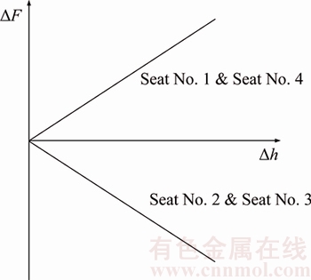
Figure 5 Variation curves of secondary spring loads with shims added to seat No. 1

solved in this loop and i as a counting variable. Initialize △h_i and i.

2) Calculate the sum of F₀₁ and F₀₄. Name it as F₁₄ and then obtain F₂₃ similarly. Solve the objective function J by Eq. (28).

3) Compare F₁₄ with F₂₃. If F₂₃ is larger, increase the value of △h₁ and △h₄ by a small step averagely; otherwise do this operation to △h₂ and △h₃ instead.

4) Calculate the new value of F_i by Eq. (19). Update F₁₄ and F₂₃ with F_i.

5) Solve the new value of J. If J decreases, which means that a better solution has been obtained, record △h_i as the current optimal shim quantity sequence. Let i=0 and go to step 6). Otherwise let i=i+1 and go to step 7).

6) Calculate h_i where h_i=h_i+△h_i. Note that h_i should be less than △H_max all the time; otherwise end the loop directly.

7) To avoid the searching process falling into a local minimum easily, a special operation based on the idea of momentum term [17, 18] is designed as follows: if i≤5, still choose points for shimming and update Δh_i as is done in step 3), then return to step 4) to go on searching; otherwise end the loop and output the optimal shim quantity sequence solved by this algorithm. Since the extra searching works similarly to the momentum parameter commonly used in artificial neural networks [19, 20], it is named as the momentum operation figuratively.

The flow chat of this gradient-based algorithm is shown in Figure 6.

Note that it is just an inner loop of the whole optimal method demonstrated in Figure 3, aiming to find the optimal shim sizes through simulation. The output will then be used in the shimming experiment on the test rig in Figure 2 for further verification, after which new spring load distribution would be obtained for the best regulation discrimination.

Figure 6 Flowchart of gradient-based algorithm

6 Experiments and discussion

6.1 Verifying tests on modification

Following the instructions of equivalent stiffness acquisition in Section 4.3, experiments are done on No. 202 car body of locomotive HXD1B. Figure 7 shows the fitting result of spring No. 1.

Equivalent stiffness of all secondary springs together with the nominal stiffness are shown in Table 1. As we can see, the largest deviation between these two kinds of stiffness is 8.45%. Undoubtedly, the modification is quite essential.

Matrix K could be modified with the equivalent stiffness by Eq. (26). Table 2 shows matrices of No. 202 car body before and after modification of the spring stiffness.

To demonstrate the effectiveness of this modification more clearly, an extra experiment was done as follows: raise the actuator under spring No.1 step by step; record the load and rising height after each operation as the experimental results.

Figure 7 Linear regression result of equivalent stiffness of spring No. 1

Table 1 Stiffness of secondary springs in No. 202 car body

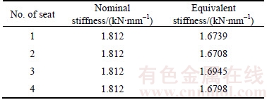
Table 2 Matrix K of No.202 car body before and after modification

Correspondingly, those two matrices in Table 2 are utilized for the spring loads prediction as calculation results before and after modification, respectively. Comparison of these results can be seen in Figure 8.

As is shown, the forecasting model after modification works more accurately on prediction. For a better illustration, the root mean square error is used to measure the effectiveness of those two models, which decreases significantly from 0.1129 kN to 0.0787 kN after modification. Similar laws have been observed on other springs, too. The improvement is 28% on average for car bodies of locomotives HXD1B.

Figure 8 Calculation and experimental results

6.2 Experiments on gradient-based algorithm

Experiments are done on the No. 202 car body. With help of matrix K, the gradient-based algorithm is used to find the optimal shim quantity sequence. Here we set the maximum shim size ΔH_max as 10 mm and the initial shim sizes as 0 mm. Since the thickness of shim added to a seat in application is too large for a step, 0.05 mm is utilized instead. Experimental results are shown in Table 3 and the search process can be seen in Figure 9.

Table 3 Experimental results of gradient-based algorithm on No. 202 car body

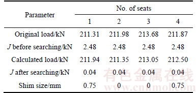
As reported in Table 3, the value of objective function J decreases dramatically from 2.48 kN to 0.04 kN with 0.75 mm thick shims both added to seat No. 1 and No. 4. Figure 9 shows clearly the efficiency of the gradient-based algorithm which solves the optimal shim quantity sequence in less than 30 steps. Effectiveness of the momentum operation is also shown in this figure.

Figure 9 Search process of gradient-based algorithm

Interestingly, decreasing from 0.73 kN² to 0.40 kN², secondary spring load variance follows the trend of J shown in Figure 9, which can be seen in Figure 10. This illustrates that even though Eq. (6) is just a necessary condition for the best regulation of load distribution, it still gives a very effective guidance for the adjustment.

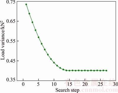
Figure 10 Trend of spring load variance during search process

6.3 Experiments on whole method for secondary spring load equalization

As demonstrated in Figure 3, Section 6.2 shows results of the optimal shim quantity sequence quantity determination clearly. For verification of the effectiveness of the whole method for secondary spring load equalization, further experiments should be conducted on the test rig shown in Figure 2 through shimming procedure.

In practical application, shims are usually added to one seat of four when it is possible for the workloads reduction. Generally speaking, it is the seat with less secondary spring load or fewer added shims that will be considered first. Moreover, the thinnest shim in actual shim adding application is 0.5 mm thick, hence an approximation of the solved value will be utilized instead. In terms of the experiment in Section 6.1, 1.5 mm thick shims will be added to seat No.1 for actual shim adding operation on the test rig. Adjustment results are shown in Table 4.

As we can see in Table 4, reduced from 0.73 kN² to 0.54 kN², the secondary spring load distribution becomes much better after shim adding operation on the test rig. It is reasonable that there is a certain deviation between simulation results in Table 3 and actual results in Table 4, since some errors are unavoidable during model establishment, modification and application.

Table 4 Secondary spring load distribution after shim adding operation on test rig

In this sense, the optimal method proposed above for secondary spring load equalization does perform efficiently in practice. For further verification, experiments are done on several other types of railway vehicles in China, including locomotives of the B0–B0 axle arrangement as well as metro trainsets. Note that the secondary spring load forecasting model needs to be re-established and re-modified for each type of car body. Adjustment results are shown in Table 5.

As reported in Tables 4 and 5, secondary spring load variances of these five car bodies are reduced by 26%, 17%, 51%, 76% and 75%, respectively, illustrating well the effectiveness and reliability of this regulation method for multiple types of railway vehicles.

It is also impressive and reasonable that the adjustment results are more significant for car bodies of locomotive SS4 and the tested metro vehicle, since original load distributions of them are worse due to their quite different secondary suspension structures.

Table 5 Adjustment results of different types of railway vehicles

7 Conclusions

Devoted to the improvement of secondary spring load distribution of railway vehicles with two-stage suspension, an effective and reliable method is proposed in this paper based on three main studies below:

1) The best regulation of secondary spring load distribution is determined by the mass center of car body. The proposed necessary condition gives an effective guidance for the load equalization adjustment.

2) The relationship between secondary spring loads and the shim quantity sequence is revealed by the secondary spring load forecasting model. Modification based on the study of equivalent stiffness of secondary springs increases its accuracy dramatically.

3) The optimization model for secondary spring load adjustment with the gradient-based algorithm could solve the optimal shim quantity sequence efficiently. Experiments on multiple types of car bodies have shown the feasibility and efficiency of proposed modeling and regulation method.

4) This paper succeeds to provide an important and basic guidance for secondary spring load equalization through shimming procedure, contributing to the running safety of railway vehicles effectively.

References

[1] PAN D F, WANG M G, ZHU Y N, HAN K. An optimization algorithm for locomotive secondary spring load adjustment based on artificial immune [J]. Journal of Central South University, 2013, 20(12): 3497–3503.

[2] General Administration of Quality Supervision, Inspection and Quarantine of the People’s Republic of China, Standardization Administration of the People’s Republic of China. General technical specification for electric locomotive [M]. Beijing, China: China Zhijian Publishing House, 2007. (in Chinese)

[3] BS EN 14363: 2005. Railway applications-Testing for the acceptance of running characteristics of railway vehicles testing of running behavior and stationary tests [S]. 2007.

[4] International Electrotechnical Commission. Railway applications-rolling stock–testing of rolling stock on completion of construction and before entry into service (CEI/IEC61133: 2006) [M]. Geneva, Switzerland: IEC Central Office, 2006.

[5] BELOBAEV G Y. Adjustment of the spring suspension mechanism of ТЭМ3type diesel locomotive [J]. Foreign Diesel Locomotive, 1988(10): 50-52. (in Chinese)

[6] CURTIS D L, SKRZYPCZYK W G, THOMAS T J. Method of adjusting the distribution of locomotive axle loads: US, US 4793047 A [P]. 1988.

[7] RUZHEKOV T, DIMITROV E. Influence of locomotive spring system parameters on difference of static loading of its running wheels [M]. IEZT, Bulgaria, 1984: 99–113.

[8] NENOV N G, DIMITROV E N, MIHOV G S, RUZHEKOV T G. Electronic system of measuring locomotive wheels load and defining operations necessary to minimize existing differences [C]// 2006 29th International Spring Seminar on Electronics Technology. St. Marienthal, Germany: IEEE, 2006: 219–224.

[9] TANAKA Y. Utilization of a static wheel load calculation program for the wheel load adjustment work [J]. Japan Society of Mechanical Engineers, 2002, 11: 409–412.

[10] HAN W M, MA R, ZHU S J, QIAN L M. Study and application of locomotive weighing and spring adjusting algorithm [J]. Diesel Locomotives, 2008(1): 19–22. (in Chinese)

[11] NENOV N G, DIMITROV E N, MANOEV V D, MIHOV G S. Small local network for information system of measuring railway vehicle wheel load [C]// 2009 32nd International Spring Seminar on Electronics Technology. Brno, Czech Republic: IEEE, 2009: 1–4.

[12] LUO H B, HU H P. Bogie load test bench and its application [J]. Technology for Electric Locomotives, 2001, 24(4): 39-41. (in Chinese)

[13] YANG Z X, PAN D F, LONG X B, JIANG L H. Development of the testing bench for the inspection of the locomotive body and adjustment of coil springs [J]. Locomotive & Rolling Stock Technology, 2006(5): 21–24. (in Chinese)

[14] PAN D F, HAN K, ZENG Y B, YANG Z X. Locomotive secondary springy load test device and its application [J]. Electric Locomotives & Mass Transit Vehicles, 2003(5): 37–39. (in Chinese)

[15] SARITAS A, KOSEOGLU A. Distributed inelasticity planar frame element with localized semi-rigid connections for nonlinear analysis of steel structures [J]. International Journal of Mechanical Sciences, 2015, 96–97: 216–231.

[16] LIMA L R O D, ANDRADE S A L D, VELLASCO P C G D S, SILVA L S D. Experimental and mechanical model for predicting the behaviour of minor axis beam-to-column semi-rigid joints [J]. International Journal of Mechanical Sciences, 2002, 44(6): 1047–1065.

[17] GUO S J, XU F, XU W C, FAN K. Weighted multi-modulus blind equalization algorithm based on momentum term [M]// Mechanical Engineering and Technology. Berlin, Heidelberg: Springer, 2012: 625–630.

[18] LIU G Q, ZHOU Z H, ZHONG H Q, XIE S L. Gradient descent with adaptive momentum for active contour models [J]. Computer Vision, IET, 2014, 8(4): 287–298.

[19] ATTOH-OKINE N O. Analysis of learning rate and momentum term in backpropagation neural network algorithm trained to predict pavement performance [J]. Advances in Engineering Software, 1999, 30(4): 291–302.

[20] SHU H, XU Y K. Application of additional momentum in PID neural network [C]// Information Science and Technology (ICIST). 2014 4th IEEE International Conference on. Shenzhen, China: IEEE, 2014: 172–175.

(Edited by HE Yun-bin)

中文导读

两系悬挂式轨道交通车辆二系支承载荷均布方法研究：建模分析与载荷优化调整

摘要：为保障行车安全，具有两系悬挂结构的轨道交通车辆其二系支承载荷应尽可能均匀分布。然而，此类超静定结构往往存在强耦合效应，常规人工加垫调整显得繁琐而低效。为此，本文提出了一种行之有效的研究方法以指导生产实践。首先对机车车辆二系悬挂结构进行建模并作受力分析，在此基础上得出二系支承的最优载荷分布状态，作为加垫工序的调整目标。通过探索各支承下的垫片分布与载荷变化量之间的映射关系，提出了一种载荷分布预测模型，并结合试验过程中车体弹性形变状态对模型参数进行了优化。此外，为有效求解最优载荷分布以及相应加垫方案，设计了一种基于动量因子的梯度下降算法。本文研究结果为多种轨道交通车辆的二系支承载荷最优分布实验提供了重要的理论支持，通过调簧试验台及大量实车测试，验证了本文方法的有效性。

关键词：轨道交通车辆；二系支承载荷均布；最优分布调整；加垫工艺；弹性形变

Foundation item: Project(51305467) supported by the National Natural Science Foundation of China; Project(12JJ4050) supported by the Natural Science Foundation of Hunan Province, China

Received date: 2016-09-12; Accepted date: 2017-03-15

Corresponding author: HAN Kun, PhD, Associate Professor; Tel: +86–13787138625; E-mail: hkun@csu.edu.cn; ORCID: 0000-0003- 4091-327x