J. Cent. South Univ. (2016) 23: 2587-2594

DOI: 10.1007/s11771-016-3320-9

A novel algorithm for SLAM in dynamic environments using landscape theory of aggregation

HUA Cheng-hao(华承昊)¹, DOU Li-hua(窦丽华)¹, FANG Hao(方浩)¹, FU Hao(付浩)²

1. School of Automation, Beijing Institute of Technology, Beijing 100081, China;

2. College of Mechatronic Engineering and Automation, National University of Defense Technology,Changsha 410073, China

Central South University Press and Springer-Verlag Berlin Heidelberg 2016

Abstract: To tackle the problem of simultaneous localization and mapping (SLAM) in dynamic environments, a novel algorithm using landscape theory of aggregation is presented. By exploiting the coherent explanation how actors form alignments in a game provided by the landscape theory of aggregation, the algorithm is able to explicitly deal with the ever-changing relationship between the static objects and the moving objects without any prior models of the moving objects. The effectiveness of the method has been validated by experiments in two representative dynamic environments: the campus road and the urban road.

Key words: mobile robot; simultaneous localization and mapping (SLAM); dynamic environment; landscape theory of aggregation; iterative closest point

1 Introduction

Simultaneous localization and mapping (SLAM) is the process that an autonomous robot builds a consistent map of the environment as the robot moves, while simultaneously keeping track of the robot’s position within this map [1]. Accurate and robust SLAM is essential for mobile robot to accomplish autonomous navigation tasks. Since SMITH and CHEESEMAN [2] firstly proposed the probabilistic SLAM problem in 1986, a number of researchers have delved into this area and made many contributions [3]. Most of existing approaches for SLAM focus on static or small scale environment and these approaches have already made remarkable progress [4]. However, SLAM in dynamic or large scale environment is still a challenging problem [5].

In recent decade, some works began to focus on SLAM in dynamic environments. MONTEMERLO et al [6] used Rao-Blackwellized particle filter for people tracking while localizing the robot. Yet, their approach requires some prior map information. et al [7] tried to solve the problem of people detection and tracking by using sample-based joint probability data association filters (SJPDAFs). For SLAM in crowded urban environment, WANG et al [8-9] proposed a mathematical framework to integrate SLAM and DATMO (detection and tracking moving objects). Their idea is to construct a map of the dynamic environment by identifying and keeping track of the moving objects in it. However, efficient detection and tracking of moving objects is in itself a very complex problem. To distinguish the static background from the moving objects, HUANG et al [10] proposed an algorithm based on sonar temporal difference and statistical background subtraction, and incrementally build a fuzzy-tuned grid map of the environment. However, their approach does not model the odometry noise. MEYER-DELIUS et al [11] proposed a dynamic occupancy grid SLAM method based on hidden Markov model (HMM). In their approach, the parameters of the HMM is learned from the history observations. They termed their approach as lifelong localization and mapping [12-13]. Their approach is for semi-dynamic environments, such as parking lot [14-15].

Although there exists a lot of work trying to tackle SLAM in dynamic environments, it is still an unresolved problem. The key to solve this problem is an efficient approach which could identify dynamic objects from the static background. In this work, drawing inspirations from the landscape theory of aggregation [16-17], we propose a novel approach for SLAM in dynamic environments. Our method is able to explicitly distinguish the moving objects from the static background without explicitly modeling the moving objects.Our method has been validated by experiments in two representative dynamic environments: the campus area with a lot of slowly-moving pedestrians and the urban area with many fast-moving cars. Experimental results obtained with data acquired by our autonomous vehicle, demonstrate that our method is well-suited for mapping dynamic environments. Furthermore, the achievement of this work can be used on DATMO research.

2 Framework for mapping in dynamic environments

Mapping in the dynamic environment has always been a hot research topic. Although there has been a lot of research in this area, it is still an unresolved problem. Some recent works have shown that with some reasonable assumptions, this problem could be decoupled into two sub-problems: the simultaneous localization and mapping (SLAM) and the detection and tracking of moving objects (DATMO) [8]. The general probabilistic formula for mapping in dynamic environments can be described as follows:

                   (1)

where subscripts 0, 1, …, k are the discrete time index; x₀is the initial pose of the robot, which is assumed to be known; are the robot trajectory in consecutive time steps; are the locations of n moving objects that appeared inside the sensor’s perception range at time step k; M_kis the accumulated stationary background map of the environment at time step k; are the environment measurements obtained from the sensors up to time k;are the odometry measurements of the robot up to time k.

Make assumptions that the measurements of the dynamic environment can be divided into the measurements of stationary and moving objects:

                     (2)

and the measurements of moving objects carry no information about the map and the robot poses:

                (3)

We can derive the following posterior by exploiting the standard Markov assumption of robot’s motion model:

       (4)

where the sensor measurements of the stationary objects and moving objects are denoted as and respectively.

3 SLAM in dynamic environments using landscape theory of aggregation

In dynamic environments, the states of the moving objects and the relationship between static objects and moving objects are changing over time. Besides, the velocities of the moving objects are also changing. In order to tackle these challenges, the landscape theory of aggregation is introduced in this work. With the coherent explanation of how actors will form alignments in a game provided by the landscape theory of aggregation, we propose a novel algorithm to separate the stationary objects from the moving objects in dynamic environments, and then construct a consistent map of the dynamic environment.

3.1 Introduction of landscape theory of aggregation

Landscape theory of aggregation was firstly proposed by AXELROD and BENNETT [16], and was later shown to be applicable for analyzing multi-player games in political, economic, and social problems [18-19].

Landscape theory of aggregation begins with a game. For a game with n players, which are denoted by , each player A_ihas its own size s_i, whereThe size s_ireflects the importance of A_icomparing to other players. For example, if players are nations, the size of a player might be measured by the demographic, industrial or military factors, or a combination of these. Landscape theory of aggregation assumes that, each pair of players A_i and A_j has a propensity, denoted by p_ij, which measures the willingness of A_i and A_j to be in the same group. p_ij is a positive value if A_i and A_j get along well together or negative if they have many sources of potential conflicts. Obviously, propensity is symmetric, that is p_ij=p_ji.

Each of the player is placed into a unique group G_c, this is called a configuration of these n players. For a given configuration where m is the number of groups, 1≤m≤n, landscape theory of aggregation defines the distance between any two players d_ij(G)as follows:

For any denote:

                           (5)

                       (6)

If two players are in the same group, the distance between them is 0. If they are in different groups, their distance is 1. For a given configuration G, the frustration of a player A_i is defined as

                        (7)

If A_i wants to minimize its frustration, it must ensure that: A_i is in the same group with those players who have positive propensity with A_i, since otherwise p_ij>0 and d_ij(G)>0; A_i is in a different group from those players with whom it has a negative propensity to align, since this would make d_ij(G)>0 when p_ij<0.

The frustration of the entire configuration G is the weighted sum of the frustrations of each player in that configuration, where the weights are the size of the players:

                            (8)

             (9)

E(G)is also called the energy of the configuration G. The energy of every possible configuration will construct an energy landscape. In this energy landscape, every point represents a possible configuration with its energy value. Using this energy landscape, the global minimum and local minima could be found, which represent the stable partitions of the n players. Minima also mean the equilibriums of the game. From a given starting configuration, landscape theory of aggregation can predict how the configuration will change according to the principle of downward movement to an adjacent configuration. Consequently, the stable configurations are those minima in the landscape. This is the process of “aggregation”. During the aggregation process, highly compatible elements tend to be gathered and less compatible elements tend to be apart. Mathematically, the landscape theory of aggregation can be formulated in terms of a constrained optimization problem as follows:

minE(G) subject to,

                   (10)

3.2 SLAM in dynamic environments using landscape theory of aggregation

We introduce the landscape theory of aggregation theory to solve the problem of dividing the robot’s environment measurements Z_0:kinto stationary objects and moving objects To meet the requirements of SLAM in dynamic environments, the landscape theory of aggregation theory have been modified in the following aspects: the theoretical formula, the application and the solving method.

Firstly, by looking at Eq. (7), we noticed that it cannot reflect the importance of the players’ size. Just as stated in the landscape theory of aggregation: “...This takes account of the fact that a source of conflict with a small country is not as important for determining alignments as an equivalent source of conflict with a large country” [16]. Based on Eq. (7), when facing with the same sources of potential conflict, A_iand A_j will have the same frustration s_is_jp_ij. However, the influence to each other is not equal. Hence, we modify Eq. (7) as

                      (11)

and Eq. (9) is modified as

            (12)

Secondly, to utilize the landscape theory of aggregation in the SLAM context, we make the following new definitions.

Definition 1: Player. In the SLAM context, player is defined as the landmark or feature point A_i in the measurement scan z_kwhich needs to be assigned as belonging to stationary object or moving object. Without loss of generality, we assume that there are n feature points in the measurement scan z_k,

Definition 2: Size of the player. Size of the player is defined as the inverse standard deviation of the location changes of each feature point in z_k. This standard deviation is obtained by comparing z_k with the following scan measurements These measurements are in the local coordinate system, which have to be compared in the global coordinate system. Without loss of generality, denote the location of the feature point A_i

in global coordinate system at time k be the pose uncertainty of the robot at time k be δ_k, which incorporates both the observation uncertainty and the motion uncertainty. Thus, the normalized Euclidean distance between and could be expressed as which as termed as where is the nearest location of the feature point A_iat time k+1. From time step k to k+t, there are t distances from which we could calculate the standard deviation of these t distances. The inverse of is defined as the size s_iof player A_i. All the locations are represented in the global coordinate system of the robot.

The player size s_ishows the stationary level of the player A_i’s location. The more stable the A_i’s location, the larger the size.

Definition 3: Propensity between players. From time step k to k+t, the similarity between player A_iand A_j can be evaluated by a series of distances in consecutive time steps:

, …,

Hence, the propensity between player A_iand A_j is defined as

              (13)

Theoretically, the value of p_ijranges from -∞ to 1. In practice the value of p_ij can not deviate too far away from 0, as the value of in practice wouldn’t be far away from 1. This definition guarantees that p_ij is a large positive value if player A_iand A_j have similar stationary or movement levels, and otherwise a large negative value.

Definition 4: Other concepts. The other concepts, including the configuration G, the frustration (energy) of the configuration G, the distance d_ij(G)between any two players A_iand A_j under a specific configuration G, and the frustration of each player, could be directly transferred from the landscape theory of aggregation. Those definitions could be obtained from Eqs. (5), (6), (11), and (12).

Particularly, in any configuration of our problem, there are only two groups: one contains all the stationary feature points and the other contains all the moving feature points. Accordingly, the problem of dividing the robot’s environment measurements Z_0:kinto stationary objects and moving objects can be formulated as a constrained optimization problem:

subject to,

       (14)

Thirdly, to solve the constrained optimization problem of formula (10), the original landscape theory of aggregation uses genetic algorithm [16-19]. However, in our case, as the number of feature points, defined as n in Eq. (14), is usually in an order of a few thousands, the genetic algorithm might not be directly applicable. An example of the feature points in a scan of laser range finder is shown in Fig. 1.

Notice that, although the value of n is large, the group number m is as small as 2, which represents the stationary objects group and the moving objects group. Based on this characteristic, in solving Eq. (14), we cast the problem as a two-class classification problem.

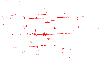
Fig. 1 Feature points in a laser scan

The initial stationary objects group is obtained from those feature points whose location variations are always smaller than the robot uncertainty. Those feature points with a larger location variation constitute the initial moving objects group.

Mathematically, the initial stationary objects group could be expressed as

                  (15)

The initial moving objects group could be expressed as

                  (16)

From the view of landscape theory of aggregation, those training samples provide a proper initial configuration for the aggregation process, which could speed up the searching process for the global minimum. With these initial samples and iteratively utilizing Eq. (11), other feature points will be classified either in the stationary objects group or in the moving objects group. Thus, we obtain the solution of Eq. (14). As a result, the SLAM in dynamic environments problem could be converted into conventional SLAM in static environments problem:

          (17)

Expression (17) is the summary of our algorithm for SLAM in dynamic environments using landscape theory of aggregation.

Algorithm 1: SLAM in dynamic environments using landscape theory of aggregation

Inputs: Initial pose of the robot x₀, robot’s environment measurements Z_0:k, robot’s moving measurements U_1:k, uncertainties of the robot’s pose δ_0:k.

Outputs: Stationary objects and moving objects in the environment, the map M_kof the dynamic environment.

Step 1) Transform Z_0:k into the global coordinates using x₀ and U_1:k.

Step 2) Compare z_awith the following t scan measurements

For a=0 k do

For all feature points A_i in z_ado

Calculate the normalized location changes of A_i:

.

Calculate the standard deviation of these t distances as

Calculate the size of A_i,

Calculate the propensity p_ij between A_i and any other points A_j in z_a using formula (13).

End for

Evaluate the energy landscape of z_a by the constrained optimization of formula (14).

Find the initial stationary objects group and the initial moving objects group in z_a using formulas (15) and (16).

Classify other feature points by formula (11), while expanding the two initial groups incrementally.

Obtain stationary objects and moving objects in z_a.

End for

Step 3) Convert the SLAM in dynamic environments problem into the SLAM in static environments problem

by introducing the stationary objects .

Step 4) Solve by conventional algorithm for SLAM in static environments.

Step 5) Obtain the result map M_k of the dynamic environment.

4 Experimental results

We tested our algorithm in two representative dynamic environments: the campus environment with walking pedestrians and few vehicles in relatively low speed, the urban environment with lots of vehicles with relatively high speed. Experimental data are collected by our autonomous vehicle which is equipped with novatel inertial measurement unit (IMU) device, a GPS receiver, and a laser rangefinder. The motion uncertainty could be obtained from the parameters of the IMU, and the observation uncertainty is determined by the resolution of the laser rangefinder. As the detection range of the laser rangefinder is up to 80 m, we run our algorithm whenever the vehicle moves around 12 m. Therefore, we can get appropriate measurement scans for identifying stationary objects and moving objects in the environment.

Figures 2(a)-(c) show three adjacent observation scans in a dynamic environment and Fig. 2(d) shows the results of projecting these three scans into the same global coordinate. Here, we directly use the IMU output to project all these three scans. It is observed that the stationary objects, including the road boundaries, maintain the same across all these three scans, while the moving cars move remarkably.

We also compared our algorithm with the classical K-means clustering algorithm. Figure 3 shows the results of the identified stationary objects obtained by the K-means algorithm and our proposed approach. It is observed that by using our algorithm, most of the moving objects are filtered out, while the result of K-means still contains some moving objects.

Once the stationary objects and the moving objects are classified by the algorithm proposed in this work, we employ iterative closest point (ICP) algorithm which only performs on the static objects, to register neighboring scans and generate a map of the surrounding scene.

Figure 4 shows the map generated by our proposed method in the campus environment. Figure 4(a) shows an aerial photo of the campus, while Figs. 4(b) and (c) show the result map of ICP with and without our algorithm.

Figure 5 shows the trajectories obtained by the integrated GPS/IMU device, which could be considered the ground truth, together with the trajectories obtained by our proposed approach and the results obtained by the raw ICP approach. It is clearly seen that the drift error of the proposed approach is much smaller than the original ICP approach. This is mostly due to the fact that we removed the moving objects which would otherwise be noise for the ICP approach.

We also did experiments in the urban area which contains a lot of fast moving vehicles. The obtained trajectory of our method is shown in Fig. 6, which also shows the GPS trajectory and the trajectory of original ICP without removing moving objects. It is also seen that our method performs much better than the original ICP approach. The resulting map of our method is shown in Fig. 7. It can be seen that most of the moving objects have been filtered out. The resulting map of the original ICP is shown in Fig. 8.

From the above experiments, it is clearly seen that our proposed approach could effectively identify the moving objects. By removing these moving objects, our proposed approach essentially performs as a pre- processing step, which could boost the performance of any scan registration approaches. The results of these experiments illustrate the effectiveness and the validity of our proposed method for different dynamic environments.

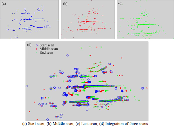
Fig. 2 Representation of three adjacent observation scans:

Fig. 3 Comparison of identification results of static objects:

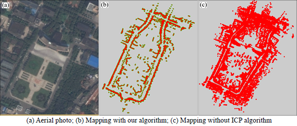
Fig. 4 Comparison of mapping results:

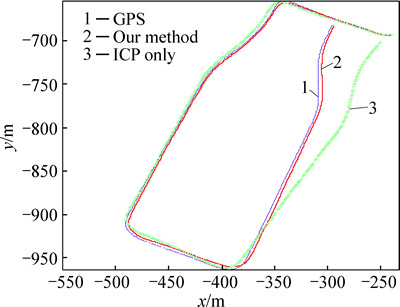
Fig.5 Comparison of location trajectories in campus

Fig. 6 Comparison of location trajectories in urban road

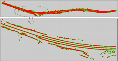
Fig. 7 Mapping result of our method (up) and a zoomed in view (below)

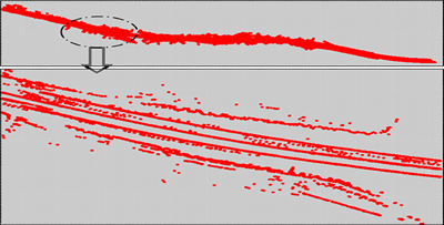
Fig. 8 Mapping result of original ICP approach (up) and a zoomed in view (below)

5 Conclusions

We presented a novel approach for SLAM in dynamic environments. It utilizes the landscape theory of aggregation to distinguish the stationary objects from the moving objects in dynamic environments, and then build consistent maps of the dynamic environments. Our approach provides a principled way to deal with the changing relationship between the static objects and the moving objects without any prior models of the moving objects. We evaluated our approach using real-world data obtained from two representative dynamic environments. The results demonstrate that our method is well-suited for mapping dynamic environments.

Extending from current work, solving method for searching global minimum of landscape in this work can be improved, while maintaining computational efficiency. Additionally, we would like to apply the achievement of on DATMO in future research which is necessary for autonomous navigation in dynamic environments.

References

[1] DURRANT-WHYTE H, BAILEY T. Simultaneous localization and mapping: Part I [J]. IEEE Robotics & Automation Magazine, 2006, 13(2): 99-110.

[2] SMITH R C, CHEESEMAN P. On the representation and estimation of spatial uncertainty [J]. International Journal of Robotics Research, 1986, 5(4): 56-68.

[3] CHEN Bai-fan, CAI Zi-xing, HU De-wen. Approach of simultaneous localization and mapping based on local maps for robot [J]. Journal of Central South University of Technology, 2006, 13(6): 713-716.

[4] LI Yang-ming, LI Shuai, GE Yun-jian. A biologically inspired solution to simultaneous localization and consistent mapping in dynamic environment [J]. Neurocomputing, 2013, (104): 170-179.

[5] PETROVSKAYA A, THRUN S. Model based vehicle detection and tracking for autonomous urban driving [J]. Autonomous Robots, 2009, 26(2/3): 123-139.

[6] MONTEMERLO M, THRUN S, WHITTAKER W. Conditional particle filters for simultaneous mobile robot localization and people-tracking [C]// IEEE International Conference on Robotics and Automation, ICRA. 2002. Wachington DC: IEEE, 2002: 695-701.

[7] D, SCHULZ D, BURGARD W. Mobile robot mapping in populated environment [J]. Advanced Robotics, 2003, 17(7): 579-597.

[8] WANG C C, THORPE C, THRUN S. Online simultaneous localization and mapping with detection and tracking of moving objects: Theory and results from a ground vehicle in crowded urhan areas [C]// IEEE International Conference on Robotics & Automation, ICRA. Taipei: IEEE, 2003(1): 842-849.

[9] WANG C C. Simultaneous localization, mapping and moving object tracking [J]. International Journal of Robotics Research, 2007, 26(9): 889-916.

[10] HUANG G Q, RAD A B, WONG Y K. A new solution to map dynamic indoor environment [J]. International Journal of Advanced Robotic Systems, 2006, 3(3): 199-210.

[11] MEYER-DELIUS D, BEINHOFER M, BURGARD W. Occupancy grid models for robot mapping in changing environment [C]// Proc of the AAAI Conf on Artificial Intelligence. Toronto, Ontario: AAAI, 2012: 2024-2030.

[12] TIPALDI G D, MEYER-DELIUS D, BEINHOFER M, BURGARD W. Lifelong localization and dynamic map estimation in changing environment [C]// RSS Workshop on Robots in Clutter. Berlin: RSS, 2012: 80-81.

[13] TIPALDI G D. LifeNav-reliable lifelong navigation for mobile robots [EB/OL]. [2015-10-21]. http://www.lifelong- navigation.eu/.

[14] TIPALDI G D, MEYER-DELIUS D, BURGARD W. Lifelong localization in changing environment [J]. International Journal of Robotics Research, 2013, 32(14): 1662-1678.

[15] MAZURAN M, BURGARD W, TIPALDI G D. Nonlinear factor recovery for long-term SLAM [J]. International Journal of Robotics Research, 2016, 35(1): 50-72.

[16] AXELROD R, BENNETT D S. A landscape theory of aggregation [J]. British Journal of Political Science, 1993, 23(23): 211-233.

[17] AXELROD R M. The complexity of cooperation: Agent-based models of competition and collaboration [M]. Princeton, New Jersey: Princeton University Press, 1997.

[18] AXELROD R, MITCHELL W, THOMAS R E, SCOTT BENNETT D, BRUDERER E. Coalition formation in standard-setting alliances [J]. Management Science, 1995, 41(9): 1493-1508.

[19] SUGANUMA S, HUYNH V N, NAKAMORI Y, WANG S. A fuzzy set based approach to generalized landscape theory of aggregation [J]. New Generation Computing, 2005, 23(1): 57-66.

(Edited by YANG Hua)

Foundation item: Project(XK100070532) supported by Beijing Education Committee Cooperation Building Foundation, China

Received date: 2016-03-08; Accepted date: 2016-06-21

Corresponding author: HUA Cheng-hao, PhD candidate; Tel: +86-10-68912463; E-mail: huachenghao@bit.edu.cn