Trans. Nonferrous Met. Soc. China 27(2017) 2682-2690

Open pit waste removal optimization through equipment fleet scheduling

Xiao-wei GU¹, Qing WANG¹, Xiao-chuan XU¹, Jian-ping LIU^1,2, Tai-wei SUN¹, Kun DU¹

1. College of Resource and Civil Engineering, Northeastern University, Shenyang 110819, China;

2. Dongmei Foundation Company of Shenyang, Shenyang 110016, China

Received 12 December 2016; accepted 8 June 2017

Abstract: A neighborhood search algorithm was proposed to simultaneously schedule the waste removal quantity and the equipment fleet profile over the mine life for open pit mines. An initial search domain was first defined and a good schedule was obtained as the current best schedule by searching in this domain. Then, progressively narrower neighborhood search domains were constructed around the current best schedule to search for better schedules. The objective is to minimize the present value of waste removal costs over the mine life. The resulting schedule from this algorithm provides a complete fleet profile for each year over the mine life: the selected equipment models, the number of equipment units of each model, the age of each unit, as well as the quantity of waste removed. A numerical example of application was provided to demonstrate the feasibility and merits of the algorithm.

Key words: open pit; waste removal; equipment fleet; scheduling; neighborhood search

1 Introduction

Having an effective long-term production schedule and assigning proper fleets of mining equipment to fulfill the schedule are crucial to an open pit operation’s economic outcome. Consequently, great research efforts have been devoted to these topics with the aim of obtaining optimal solutions.

The long-term open pit production scheduling problem (LTOPSP) consists of determining the quantity and sequence in which the blocks should be mined in each year over the mine life, so that the overall net present value is maximized. Various approaches have been proposed to get optimal solution to the LTOPSP. Linear programming has been a popular approach where the LTOPSP is usually formulated into mixed integer programming (MIP) or pure integer programming (IP) models [1-4]. The sheer size of such models prohibits the straightforward application of standard solution techniques, and much effort has been spent on finding ways of solving the models in acceptable time frames. Two ways of block aggregation [5,6] and Lagrangian relaxation [7,8] frequently appear in the literatures. Dynamic programming is another frequently used approach to the LTOPSP [9-11]. A relatively new development in this area is the incorporation of geological and market uncertainties in solving the LTOPSP [12-15].

Fleets of mining equipment must be operated to carry out the scheduled production. Materials handling takes a lion’s share of the total equipment requirement, in terms of both capacity and cost outlay. According to Refs. [16,17], haulage cost constitutes 50%-60% of the total operating cost, and the capital cost of a truck-shovel system is in the order of hundreds of millions of US dollars for large operations. Therefore, the truck-shovel system has been the subject of extensive research to address various issues, including fleet sizing and scheduling.

Queuing network models have been used to obtain performance parameters of open pit truck-shovel  systems. Analyses of these parameters may indicate deficiencies in the system and suggest improvement measures. By solving queuing network models for different truck-shovel fleet configurations, the best fleet configuration can be found for an operation. Some examples of publications in this area can be found [18-21]. Simulation is also a widely used tool for analyzing the performance of open pit truck-shovel systems. Through many runs of simulation, statistics on performance measures of a truck-shovel system can be obtained and analyzed to pinpoint bottlenecks and to devise possible improvements. Sensitivity analyses may be conducted using simulation with respect to certain system configurations in an attempt to optimize the system. A large number of publications in this area exist, and these are some examples of recent ones [22-25].

Fleet scheduling in open pit mines mainly concerns the determination of the number and models of trucks and shovels to be used in each period to meet the scheduled production targets. BURT et al [26,27] formulated the fleet scheduling problem as a MIP model. The model determines the number and models of trucks and loaders as well as their purchase and salvage  policies, and allocates the trucks to routes and the loaders to mining locations. The objective is to minimize the present value of materials handling cost while meeting the scheduled production requirements. TOPAL and RAMAZAN [28] also used a MIP formulation to schedule truck fleet, with an objective of minimizing the overall discounted maintenance cost while achieving the scheduled production targets. FU et al [29] extended this formulation to incorporate new truck purchase. TOPAL and RAMAZAN [30] used stochastic IP to schedule the truck fleet by treating the truck maintenance cost as a stochastic parameter.

Although a large number of publications exit on the open pit production and equipment fleet scheduling problems, the two problems have been treated separately. In fact, they are closely interrelated and can be seen as the same and one problem, because the quantity of material mined (the production) in each period is normally equal to the capacity of the mining equipment fleets operating in that period, unless the mine operator is willing to let some of the available equipment capacity be idle. Separate, optimal solutions to the two problems will not be optimal when the two are considered together. Therefore, production and equipment fleet should be scheduled together or, putting it another way, production should be scheduled through equipment fleet scheduling. Unfortunately, very few publications addressed the problem in such a way. WANG et al [31] solved the waste removal and truck fleet scheduling problem as a whole, but used a fixed truck replacement rule and allowed only a single truck model. GODOY and DIMITRAKOPOULOS [32] proposed a production scheduling approach that considers the purchase cost of added equipment capacity and the ownership cost of idle capacity. This approach implicitly incorporates equipment feet sizing in production scheduling, but the fleets are represented by capacities rather than specific equipment units.

In this work, an optimization approach was presented, where open pit waste removal scheduling and equipment feet scheduling were integrated. The approach can deal with heterogeneous fleets, preexisting equipment, and considers the effective capacity and operating cost of an equipment unit as discrete functions of its age. The objective is the minimization of discounted waste removal costs.

2 Waste removal problem and its solution domain

In open pit mines, sufficient quantity of waste must be removed each year to expose enough ore to meet the ore production target. Figure 1 shows an illustration of the relationship between waste removal and ore mining, where the ultimate pit is not divided into intermediate pits as commonly practiced in China. One can see that waste (w) must be removed with the mining of ore (q). For given annual ore productions, the required quantity of waste removal may vary dramatically over the mine life, depending on the orebody geometry, the ultimate pit, the topography, and the working slope α. Supposing that the annual ore production is a constant equal to the throughput of the processing plant, the required annual waste removal may vary with time as shown by the solid curve in Fig. 2. For given orebody geometry, the ultimate pit and topography, this waste removal curve depends on the working slope, α, which in turn depends mainly on the working bench width b. The smaller the b is, the higher the α is, and the more waste will be postponed in most cases. The steepest feasible working slope corresponds to the minimum b required for operating mining equipment at normal efficiency. We use the term required waste removal to refer to the quantity of waste to be removed to meet the specified ore production with the minimum b.

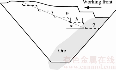
Fig. 1 Illustration of relationship between ore mining and waste removal

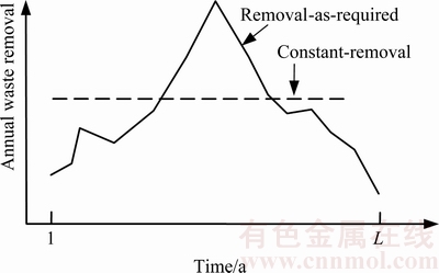
Fig. 2 Illustration of removal-as-required and constant-removal scenarios

It seems that accomplishing just the required waste removal each year over the mine life (the solid curve in Fig. 2) would be the best schedule since, according to the above definition, the waste removal is postponed as much as possible. However, this remove-as-required scenario usually results in a large increase in equipment fleet size to meet the peak capacity demand, and many equipment units will be no longer needed after the peak years. This is obviously not the best schedule considering the very high capital cost of mining equipment. This shortcoming is completely overcome if a constant amount of waste is removed each year (the dashed line in Fig. 2). But this constant-removal scenario means very high removal rates in the early years and, consequently, high early expenditure on equipment capital and operating costs.

Figure 3 shows the cumulative waste removal curves for the two scenarios when the ore production rate is constant. Any schedule falling below the removal-as- required curve in Fig. 3 is not feasible, because it cannot expose enough ore to meet the ore production; any schedule above the constant-removal curve cannot be optimal due to the high early negative cash flows. Hence, the best schedule should be sought within the domain bounded by the removal-as-required and the constant-removal scenarios. This domain is termed here as the solution domain.

Fig. 3 Illustration of solution domain for waste removal scheduling

As reasoned above, the waste removal schedule should be optimized through equipment fleet scheduling. Therefore, the waste removal optimization problem can be stated as determining the best equipment fleet for each year over the mine life, so that the total present value of waste removal costs is minimized and the cumulative quantity of waste removal at the end of each year falls in the solution domain.

3 Neighborhood search algorithm

The problem as defined above is a typical combinatorial problem. Supposing that at the start there is a preexisting fleet, F₀. We may consider replacing, salvaging different members of F₀ and adding different numbers of new equipment units of the considered models, to come up with different feasible fleets N₁ for the first year. Feasible means that the quantity of waste removed by the fleet makes the cumulative waste removal at the year end fall in the solution domain. Then, based on the feasible fleets N₁ for the 1st year, we can generate a total number of different feasible fleets N₂ for the 2nd year. This process continues until the last year of mine life. Clearly, the number of feasible fleets explodes as the time advances, and the total number of fleet combinations will be too high to be exhaustively evaluated by today’s PC computers, even for a relatively small mine.

Generating and evaluating all the feasible fleets in the above fashion is equivalent to constructing all the non-decreasing curves (schedules) in the solution domain in Fig. 3, and fitting a fleet for each year on each curve. There are theoretically an infinite number of such curves. However, considering the integer nature of equipment units and under the assumption of full utilization, only a finite number of discrete cumulative waste removal levels exist in the solution domain for each year, as represented by the dots in Fig. 3. Any curve passing one of the dots in each year represents a feasible waste removal schedule as indicated in the figure. Unfortunately, even with the discrete solution domain (DSD) represented by the dots, the number of feasible schedules is still too large for an exhaustive evaluation. Therefore, we propose a discrete neighborhood search approach to find a good solution in an acceptable time frame. The algorithm is outlined as follows.

Step 1. Define an initial search domain (ISD). The upper limit of the DSD corresponds to the constant- removal scenario which is probably the worst feasible schedule due to its high early expenditure. The best schedule is unlikely to reach this limit, except for the last year where the upper and lower limits of DSD are always the same. Therefore, the DSD can be narrowed by lowering its upper limit to define an ISD. Let W_Ut and W_Lt denote respectively the upper and lower limits of the DSD for year t. The upper limit of the ISD is set to W_IUt=W_Ut-p(W_Ut-W_Lt), where p∈(0, 1) is referred to as the domain reduction factor whose determination is explained in the numerical example.

Step 2. Divide the ISD range, [W_Lt, W_IUt]. For each year t (except the last year) into n equal segments to define n+1 search points across this range. For example, if n is 4, the size of each segment is Δ=( W_IUt-W_Lt)/4, and the cumulative waste removal levels corresponding to the 5 search points are: W_Lt, W_Lt+Δ, W_Lt+2Δ, W_Lt+3Δ and W_IUt. n+1 is referred to as the search density and denoted by n_ρ.

Step 3. A path passing one of the above defined search points in each year of the ISD forms a feasible waste removal schedule. Fit a fleet for each year on a path, so that the cumulative waste removal is the closest to that at the search point on the path at the same year, and compute the path’s present value of costs (PVC). After all the paths in ISD are evaluated, the one with the lowest PVC is selected as the current best schedule.

Step 4. Define a neighborhood search domain (NSD) with the current best schedule at its center. The NSD at each year (except the last year) consists of search points n_ρ with the mid-point on the current best schedule. For example, with n_ρ=5, the 5 search points of the NSD at year t are: W_Ot-2δ, W_Ot-δ, W_Ot, W_Ot+δ, and W_Ot+2δ, where W_Ot is the cumulative waste removal of the current best schedule at the end of year t; δ is referred to as the neighborhood increment. The NSD should not go beyond the solution domain DSD. Noted that to make W_Ot the mid-point, n_ρ must be odd.

Step 5. Fit fleets for all paths in the NSD and compute their PVCs to select the best path. If this best path is better than the current best schedule, it becomes the current best schedule; otherwise, the current best schedule does not change.

Step 6. Take a smaller δ value and repeat Steps 4 and 5, until all the predefined δ values are exhausted. The kept current best schedule is the final schedule. Reasonable δ values are explained in the numerical example.

The fleet fitting and evaluation process for a given path, in Steps 3 and 5, starts with the first year and goes forward year by year until the last year of mine life or when all the wastes have been removed. This process is outlined below.

Let W_t denote the cumulative waste removal by the end of year t on the path being processed, and the actual cumulative waste removed by the end of year t with the fleets fitted for this path (W_ft). Due to the integer nature of equipment units and the assumption of full utilization, W_ft and W_t are different for most years. The objective of fleet fitting is to find such a fleet for each year t so that W_ft is the closest to W_t. Let D_t be the required annual waste removal in year t (the solid curve in Fig. 2). Supposing that the fleet fitting process has arrived at the beginning of year t and the fleet fitted for year t-1 at its beginning is F_t-1. We now need to fit a fleet, F_t, for year t based on F_t-1. In the following description, replacement means that a used unit is replaced by a new one of the same model and the used one is salvaged; salvage means that a used unit is salvaged without replacement.

Increment the age of each equipment unit in F_t-1 by 1 and salvage those units whose ages have reached the maximum service life set for their corresponding models. The resulting fleet is the base fleet, F_bt, at the start of year t. The capacity of F_bt is Q_bt:

                          (1)

where M is the number of equipment models considered, N_m is the number of equipment units of model m in F_bt; q_mi(a_mi) is the effective capacity of the ith unit of model m with the unit's age being a_mi. With this capacity, the cumulative waste removal at the end of year t, W_bt, is

W_bt=W_ft-1+Q_bt-D_t                               (2)

Comparing W_bt with W_t, one of the following three cases will occur.

Case 1: W_bt=W_t. The capacity of F_bt exactly matches the waste removal target on the path at year t. So, the base fleet, F_bt, is taken as F_t, the feet for year t, and W_ft=W_bt. This is a very rare case.

Case 2: W_bt >W_t. The capacity of F_bt is greater than that what is targeted on the path at year t. Consider salvaging one or a combination of units in F_bt, so that the remaining fleet, F_t, has a capacity of Q_ft, which gives a cumulative waste of W_ft, with the minimum non-negative bias (W_ft-W_t). The algorithm of finding such a combination is trivial and not described. If salvaging a single unit with the smallest capacity alone makes W_ftt, no salvage occurs and F_bt is taken as F_t and W_ft=W_bt.

Case 3: W_bt t. The capacity of F_bt is insufficient to meet what is targeted on the path at year t. Consider replacing some units in F_bt and/or adding certain new units of the considered models. Find the combination of used units to replace and new units to add, so that the resulting fleet, F_t, has a capacity of Q_ft, which gives a cumulative waste of W_ft, with the minimum non-negative bias (W_ft-W_t). This combination may indicate only replacing certain used units, or only adding a certain number of new units of certain models, or both. The algorithm of finding such a combination is trivial and  not described. The replaced old units (if any) are salvaged.

For t=1, two initial conditions can be handled. One is with a preexisting fleet, F₀, in which case F₀ is the base fleet, F_b1, for the 1st year and the fleet fitting logic is exactly the same as that described above. The other is with no preexisting fleet, in which case the fleet fitting logic starts with Case 3 above and fits a fleet of all new units for the 1st year.

For the final L years, the condition W_fL=W_L must be strictly met, that is, the total waste actually removed by the fitted fleets, W_fL, must be equal to the total waste in the ultimate pit, W_L. This condition is rarely met due to the integer nature of equipment units and the assumption of full utilization. When the condition is not met, the fleet, F_L, fitted for the final year is assumed to work a fraction of a whole year at its full capacity.

After a fleet is fitted for each year on a path, the calculation of PVC of the path is a straightforward matter and the equations are omitted.

4 Numerical example

A software package has been developed for the algorithm and applied to a numerical example to test the algorithm. A deposit model from a real open pit iron mine is taken to generate the required waste removal quantity. The mine has a processing plant with a throughput of 4 Mt per year which is also the planned annual ore production from the pit. The minimum working bench width is 40 m with a bench height of   15 m and a bank slope of 60°, which gives the maximum working slope of 17°. The ultimate pit is first optimized, within which a series of maximum-working-slope pushbacks are then generated with an ore increment of 200 kt. These pushbacks are then sequenced to obtain the required waste removal quantity in each year to meet the 4 Mt of annual ore production. The mine life is 17 years and the annual ore production, the required annual and cumulative waste removals are listed in columns 2 to 4 in Table 1.

The objective is to optimize the waste removal through truck fleet scheduling. Since the tonnage that can be hauled by a truck in a given time period, with its given payload and working efficiency, is a function of the travel distance, the effective capacity of a truck is commonly expressed in terms of haulage work done per year. Therefore, the required annual and cumulative waste removal tonnages are converted into haulage work as shown in the last two columns of Table 1. The waste haulage distance is assumed to vary from 3.0 to 4.2 km as the pit deepens. A piece-wise linear interpolation is used to do the conversion.

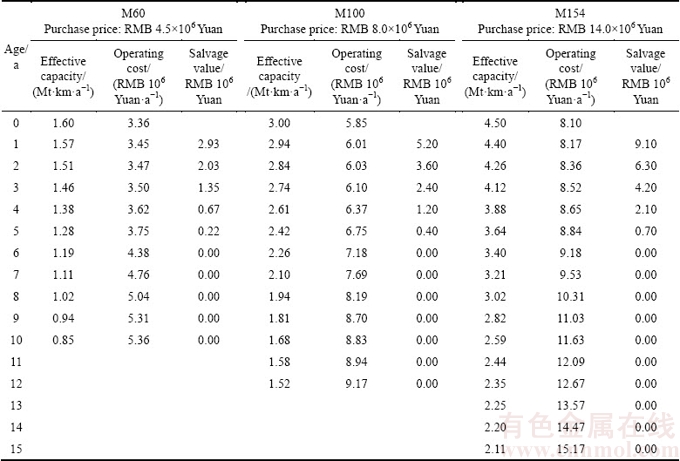
Three truck models are considered for this example with respective payloads of 60 t, 100 t and 154 t, denoted respectively as model M60, M100 and M154. Attempts were made to collect data on the effective capacities and operating costs of the trucks as functions of their ages. But the data are not in enough detail and do not cover sufficient time length to construct complete capacity and cost profiles. Therefore, the effective capacity and operating cost of each truck model were made up as discrete functions of age as given in Table 2, based on analyses on the collected data. The maximum service lives of M60, M100 and M154 are assumed to be 10, 12, and 15 years, respectively. The salvage values are based on an assumed 5 years depreciation schedule, in which the salvage values of a truck are equal to 65%, 45%, 30%, 15% and 5% of a new truck’s purchase price, after it has worked for 1 to 5 years, respectively. The new truck purchase prices are also given in Table 2.

Table 1 Required waste removal and haulage work

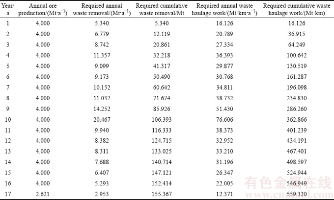
Table 2 Capacity and cost for three truck models used in example

Theoretically, any truck in an existing fleet should be considered for replacement/salvage, regardless of its age. Practically, however, no one is likely to consider replacing/salvaging a truck after it has only been in service for a couple of years. Therefore, a minimum replacement/salvage age, a_mr, is imposed for each model m in the fleet fitting process, to reduce the number of combinations to be evaluated. Two kinds of economic life for a truck model m, referred to as the static economic life and dynamic economic life and denoted by l_ms and l_md, respectively, may be considered for a_mr. The static economic life of a truck is defined as the life over which the average cost is minimum, and the dynamic economic life is the life over which the average discounted cost is minimum. Capital cost, operating costs and salvage value are all included in calculating the average (discounted) cost. Using the data in Table 2, the l_ms values for models M60, M100, and M154 are 4, 4 and 5 years, respectively. For a discount rate of 8% and a cost escalation rate of 2%, the l_md values for the three models are 7, 7 and 9 years, respectively.

The minimum replacement/salvage age, a_mr, for each model can also be user defined. Trial runs of the algorithm on different a_mr values indicated that, in the best schedules, trucks are rarely replaced/salvaged at a age beyond the range [l_ms, l_md]. Therefore, a_mr is set to l_ms for each truck model in this example.

A domain reduction factor, p, is used in the algorithm to define an initial search domain. Because minimizing PVC always tries to postpone waste  removal as much as possible, it can be reasoned that the optimal schedule would most likely lie in the lower half of the solution domain in Fig. 3 in most cases. Therefore, p=0.5 is used for this example. Note that a p value of  0.5 does not mean that all the searching will be constrained in the lower half of the solution domain, because the neighborhood search domain may go above this limit.

A series of δ values (neighborhood increments) are used in the algorithm to define neighborhood search domains. Good δ values are the capacity increase if used trucks were replaced at their corresponding minimum replacement/salvage ages, and the capacities of new trucks of the considered models. In this example, four δ values 1.60, 0.86, 0.39 and 0.22 are used, where 1.60 is the capacity of a new truck of model M60; and 0.86, 0.39 and 0.22 correspond to the capacity increase for M154, M100 and M60 if replacement occurred at their corresponding minimum replacement/salvage ages of 5, 4 and 4 years, respectively.

The search density, n_ρ, defines the number of search points to be considered in the search domain for each year. Clearly, the larger the n_ρ value is, the closer the resulting schedule should be to the unknown optimal. However, the number of schedules to be evaluated explodes with increasing n_ρ. In this example, n_ρ=3 is used.

To make the case general, a preexisting fleet of 7 trucks is assumed as given in Table 3. A discount rate of 8% and a cost escalation rate of 2% are used for PVC calculations.

Table 3 Preexisting truck fleet

Applying the above input data, the algorithm evaluated 1583540 paths, and the optimized schedule   is shown in Fig. 4, which has a PVC of  RMB 942.68×10⁶ Yuan. When fleets are fitted with the same fleet-fitting logic for the remove-as-required and constant-removal scenarios, their PVCs are RMB 987.33×10⁶ Yuan and RMB 1076.86×10⁶ Yuan, respectively.

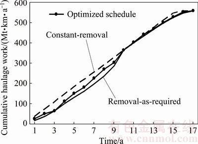
Fig. 4 Optimized waste haulage work schedule for example

The fleet profile and the waste haulage work done in each year in the optimized schedule are depicted in Fig. 5. From this figure, one can see the evolution of the truck fleet over time: the number of trucks and the model and age of each truck in the fleet for each year; the purchase and salvage/replacement time as well as the service time length of each truck. Two M60 trucks, 4 and 7 years old, in the preexisting fleet are replaced immediately at the beginning. All the trucks are salvaged/replaced before reaching their corresponding dynamic economic lives. Most of the trucks selected for the schedule is model M154. This is expected because, of the three models, M154 gives the lowest discounted capital and operating cost, when the service time length of each model is in the range [l_ms, l_md]. The peak annual haulage work in the optimized schedule is 60.7 Mt·km (see Q_ft values in Fig. 5), while the required peak is 76.606 Mt·km/a (see Table 1).

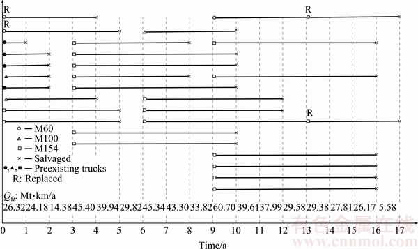
Fig. 5 Truck fleet and waste haulage work scheduled for numerical example

5 Conclusions

1) The algorithm provides not only a waste removal schedule, but also a detailed evolution of the equipment fleet profile over the mine life.

2) Different equipment model mixes can be evaluated using the algorithm to select the most appropriate ones for a given mine, making the algorithm a useful tool for both waste removal planning and equipment selection.

3) Although the equipment considered in the numerical example is trucks, loaders and drills can also be scheduled. When same equipment models are used for both waste removal and ore mining, the algorithm can do the entire production scheduling by summing up the ore mining work and required waste removal work in each year.

4) The algorithm currently does not consider equipment overhaul and the option of keeping idle equipment units when not needed temporarily. Using the current algorithm, truck and loader fleets can only be scheduled separately by independent runs. Trucks and loaders always work together and should be scheduled together with the consideration of appropriate matching between them. The execution time for the example case is 48 min. When the mine life is long, it may take an unacceptably long time to complete a run. Hence, there is a need to raise the algorithm’s efficiency. These are the issues being addressed to make the algorithm more realistic and powerful.

References

[1] GERSHON M E. Mine scheduling optimization with mixed integer programming [J]. Mining Engineering, 1983, 35: 351-354.

[2] CACCETTA L, HILL P. An application of branch and cut to open pit mine scheduling [J]. Journal of Global Optimization, 2003, 27: 349-365.

[3] RAMAZAN S, DIMITRAKOPOULOS R. Recent applications of operations research and efficient MIP formulations in open pit mining [J]. Society for Mining, Metallurgy, and Exploration, 2004, 316: 73-78.

[4] BLEY A, BOLAND N, FRICKE C, FROYLAND G. A strengthened formulation and cutting planes for the open pit mine production scheduling problem [J]. Computers & Operations Research, 2010, 37: 1641-1647.

[5] RAMAZAN S. The new fundamental tree algorithm for production scheduling of open pit mines [J]. European Journal of Operational Research, 2007, 177: 1153-1166.

[6] BOLAND N, DUMITRESCU I, FROYLAND G, GLEIXNER A M. LP-based disaggregation approaches to solving the open pit mining production scheduling problem with block processing selectivity [J]. Computers & Operations Research, 2009, 36: 1064-1089.

[7] AKAIKE A, DAGDELEN K. A strategic production scheduling method for an open pit mine [C]//Proceedings of the 28th International Symposium on Applications of Computers and Operations Research in the Mineral Industry (APCOM). Littleton, USA: SME, 1999: 729-738.

[8] KAWAHATA K. A new algorithm to solve large scale mine production scheduling problems by using the Lagrangian relaxation method [D]. Golden, USA: Colorado School of Mines, 2006: 1-217.

[9] DOWD P A, ONUR A H. Optimizing open pit design and sequencing [C]//Proceedings of the 23rd APCOM. Littleton, USA: SME, 1992: 411- 422.

[10] GU X W, WANG Q, GE S. Dynamic phase-mining optimization in open-pit metal mines [J]. Transactions of Nonferrous Metals Society of China, 2010, 20(10): 1974-1980.

[11] ERARSLAN K,  N. A simulative model for optimum open pit design [J]. Canadian Institute of Mining, Metallurgy and Petroleum (CIM) Bulletin, 2001, 94: 59-68.

[12] DOWD P A. Risk assessment in reserve estimation and open pit planning [J]. Transactions of the Institution of Mining and Metallurgy, Section A: Mining Technology, 1994, 103(9): 148-154.

[13] GHOLAMNEJAD J, OSANLOO M. Using chance constrained binary integer programming in optimizing long term production scheduling for open pit mine design [J]. Transactions of the Institutions of Mining and Metallurgy, Section A: Mining Technology, 2013, 116(2): 58-66.

[14] DIMITRAKOPOULOS R, RAMAZAN S. Stochastic integer programming for optimizing long term production schedules of open pit mines: methods, application and value of stochastic solutions [J]. Transactions of the Institutions of Mining and Metallurgy, Section A: Mining Technology, 2008, 117(4): 155-160.

[15] BOLAND N, DUMITRESCU I, FROYLAND G. A multistage stochastic programming approach to open pit mine production scheduling with uncertain geology [EB/OL]. 2008-10-24, http://www. optimization-online.org/DB_FILE/2008/10/2123.pdf.

[16] ALARIE S, GAMACHE M. Overview of solution strategies used in truck dispatching systems for open pit mines [J]. International Journal of Surface Mining, Reclamation and Environment, 2002, 16(1): 59-76.

[17] ERCELEBI S G, BASCETIN A. Optimization of shovel-truck system for surface mining [J]. The Journal of The South African Institute of Mining and Metallurgy, 2009, 109: 433-439.

[18] MUDULI P K, YEGULALP T M. Modeling truck-shovel systems as closed queuing network with multiple job classes [J]. International Transactions in Operational Research, 1996, 3(1): 89-98.

[19] KOMLJENOVIC D, PARASZCZAK J, FYTAS K. Optimization of shovel truck systems using the queuing theory [J]. CIM Bulletin, 2004, 97: 76-83.

[20] KRAUSE A, MUSINGWINI C. Modeling open pit shovel-truck systems using a machine repair model [J]. Journal of The South African Institute of Mining and Metallurgy, 2007, 107: 469-476.

[21] MAY M A. Applications of queuing theory for open-pit truck/shovel haulage systems [D]. Blacksburg, USA: Virginia Polytechnic Institute and State University, 2012: 1-72.

[22] JAOUA A, RIOPEL D, GAMACHE M. A simulation framework for real-time fleet management in internal transport systems [J]. Simulation Modelling Practice and Theory, 2012, 21: 78-90.

[23] STOUT C E, CONRAD P W, TODD C S, ROSENTHAL S, KNUDSENINT H P. Simulation of a large multiple pit mining operation using GPSS/H [J]. Journal of Mining and Mineral Engineering, 2013, 4(4): 278-295.

[24] TARSHIZI E, STURGUL J, IBARRA V, TAYLOR D. Simulation and animation model to boost mining efficiency and enviro-friendly in multi-pit operations [J]. International Journal of Mining Science and Technology, 2015, 25: 671-674.

[25] DINDARLOO S R, OSANLOO M, FRIMPONG S. A stochastic simulation framework for truck and shovel selection and sizing in open pit mines [J]. The Journal of The South African Institute of Mining and Metallurgy, 2015, 115: 209-219.

[26] BURT C. An optimisation approach to materials handling in surface mines [D]. Perth, Australia: Curtin University of Technology, 2008: 1-155.

[27] BURT C, CACCETTA L, WELGAMA P, L. Equipment selection with heterogeneous fleets for multiple-period schedules [J]. Journal of the Operational Research Society, 2011, 62(8): 1498-1509.

[28] TOPAL E, RAMAZAN S. A new MIP model for mine equipment scheduling by minimizing maintenance cost [J]. European Journal of Operational Research, 2010, 207: 1065-1071.

[29] FU Z, TOPAL E, ERTEN O. Optimisation of a mixed truck fleet schedule through a mathematical model considering a new truck-purchase option [J]. Mining Technology, Transactions of the Institutions of Mining and Metallurgy: Section A, 2014, 123(1): 30-35.

[30] TOPAL E, RAMAZAN S. Mining trucks scheduling with stochastic maintenance cost [J]. Journal of Coal Science and Engineering (China), 2012, 18(3): 313-319.

[31] WANG Q, SEVIM H, DETOMI G. A solution to the problem of scheduling and replacement in open-pit mines [C]//Proceedings of the 21st APCOM. Littleton, USA: SME, 1989: 662-673.

[32] GODOY M C, DIMITRAKOPOULOS R. Managing risk and waste mining in long-term production scheduling of open pit mines [J]. Society for Mining, Metallurgy, and Exploration, 2004, 316: 43-50.

通过设备配置优化露天矿剥离计划

顾晓薇¹，王 青¹，胥孝川¹，刘剑平^1,2，孙太伟¹，杜 坤¹

1. 东北大学 资源与土木工程学院，沈阳 110819；

2. 沈阳东煤基础公司，沈阳 110016

摘  要：给出了一个临近域搜索算法来同时优化露天矿开采寿命期的剥岩计划和设备配置计划。首先定义一个初始搜索域并在其中搜索到一个好的计划作为当前最佳计划。然后，在当前最佳计划的周围构建逐步变窄的临近搜索域，以搜索更好的计划。优化目标是使矿山寿命期的剥离成本的现值达到最小。对于矿山寿命期的每一年，由该算法求得的计划给出了完整的设备配置方案：所选择的设备型号、每种型号设备的台数、每台设备的役龄，以及剥离的废石量。以一个应用算例展示了该算法的可行性和优点。

关键词：露天矿；剥岩；设备配置；计划；临近域搜索

(Edited by Xiang-qun LI)

Foundation item: Projects (51474049, 51674062) supported by the National Natural Science Foundation of China; Project (51604061) supported by the National Science Foundation for Young Scientists of China; Projects (201202075, 2014020040) supported by the Liaoning Natural Science Founds, China; Project (LZ2014020) supported by the Liaoning Province’s Key Laboratory Construction, China; Project (20130042110012) supported by the Specialized Research Fund for the Doctoral Program of Higher Education of China; Project (F14-231-1-07) supported by the Shenyang Technical Plan Project, China

Corresponding author: Qing WANG; Tel: +86-24-83678400; E-mail: qingwangedu@163.com

DOI: 10.1016/S1003-6326(17)60297-8