J. Cent. South Univ. (2016) 23: 2630-2637

DOI: 10.1007/s11771-016-3324-5

Numerical simulation of two-phase flow in fractured porous media using streamline simulation and IMPES methods and comparing results with a commercial software

Mahmoud Ahmadpour, Majid Siavashi, Mohammad Hossein Doranehgard

Applied Multi-Phase Fluid Dynamics Lab., School of Mechanical Engineering, Iran University of Science and Technology, Tehran, Iran

Central South University Press and Springer-Verlag Berlin Heidelberg 2016

Abstract: Streamline simulation is developed to simulate waterflooding in fractured reservoirs. Conventional reservoir simulation methods for fluid flow simulation in large and complex reservoirs are very costly and time consuming. In streamline method, transport equations are solved on one-dimensional streamlines to reduce the computation time with less memory for simulation. First, pressure equation is solved on an Eulerian grid and streamlines are traced. Defining the “time of flight”, saturation equations are mapped and solved on streamlines. Finally, the results are mapped back on Eulerian grid and the process is repeated until the simulation end time. The waterflooding process is considered in a fractured reservoir using the dual porosity model. Afterwards, a computational code is developed to solve the same problem by the IMPES method and the results of streamline simulation are compared to those of the IMPES and a commercial software. Finally, the accuracy and efficiency of streamline simulator for simulation of two-phase flow in fractured reservoirs has been proved.

Key words: two-phase flow; porous media; fractured reservoirs; streamline simulation; dual porosity; implicit pressure-explicit saturation

1 Introduction

Increased global demand for fossil fuels presents Iran’s role as one of the largest holders of oil and gas reserves. Much of Iran's hydrocarbon reservoirs are fractured and the recovery rate of these fields is generally lower than other traditional reservoirs [1]. Therefore, research and development of methods for recovery from fractured reservoirs is of utmost importance in order to increase oil production. Fractured porous media is an environment cut by a network of connected fractures or channels. Since the size of reservoir can be extended to several kilometers, averaged properties of the medium are used in the mathematical model in order to simulate the flow. The geological details and computations required for flow simulation in fractured reservoirs are more complex than conventional reservoirs. In addition, fluid flow mechanism in adjacent fractures and porous media is completely different than the mechanisms in conventional porous regions. For these reasons, fluid flow is considered in two separate parts in order to model fractured reservoirs: 1) Fractures with high permeability and low porosity factor that contains small volume of fluid and transfers large amount of fluid; 2) matrix with low permeability and high porosity that contains large volume of fluid but its ability to transfer fluid is very small compared to fractures. These two parts interact with each other and the fluid of matrix can enter into fracture (and vice versa) and transfer through them [2]. Two different models have been proposed to model the fractured porous media [3]:1) Dual porosity, single permeability model (DPSP); 2) Dual porosity, dual permeability model (DPDP). According to low permeability of matrix, DPSP model can obtain results with proper accuracy; hence, in this work, the DPSP model is employed in order to simulate flow in fractured reservoirs [4].

According to the complexity of fractured reservoirs, simulation of fluid flow in reservoirs at field scale which has many geological complexities [5] is very time consuming and costly using the traditional commercial software. This issue will be very impressive for problems like optimization and history matching issues, in which a large number of simulations must be done.

BATYCKY et al [6] proposed the streamline simulation method in order to simulate waterflooding process in a heterogeneous field. They confirmed the performance and accuracy of the streamline simulation comparing results of this method with those of a commercial software [7]. After that, this method has been developed in order to simulate different fluid models and much research has been done on this technique.

Streamline simulation can be a good alternative to conventional simulators as a result of its high computational speed, low memory required for computation and proper accuracy. In this method, the pressure equation is solved on an Eulerian grid and then the speed is calculated using Darcy’s law and streamlines are traced using the Pollock’s approach [8]. The fluid properties are mapped on streamlines from the Euler grid and saturation equations are solved along the one- dimensional streamlines through defining a new parameter called time-of-flight (TOF) [6]. Finally, the results obtained on streamlines are mapped back to the Eulerian underlying grid and the process is repeated until the end of simulation time [9].

The so IMPES method is one of the methods which is commonly used to simulate multi-phase flows in porous media. In this method, the pressure equation is implicitly solved and then saturation equation is explicitly discretized and solved. In this work, in addition to the in-house streamline simulator, an in-house computational code based on the IMPES technique is developed to simulate two-phase flow of oil-water in naturally fractured porous media, in order to compare the results of both methods with each other carefully, and also compare them with the results of a commercial software.

In the next sections, after introduction of the governing equations of two-phase flow in fractured porous media, the theory of streamline simulation and the equations and corresponding assumptions used are presented. In addition, the IMPES simulation technique is described. Then, defining a problem, the simulation results of streamline method and the IMPES method as well as the results of the commercial software are assessed and compared with each other.

2 Governing equations

The problem that has been addressed in this work is a horizontal reservoir, a 2D geometry, and therefore the gravity is ignored. The compressibility of both fluid and rock and the effect of capillary pressure are neglected in fractures. In addition, according to the assumptions made for the dual porosity, single permeability model, it is assumed that fluid does not flow directly from a block matrix to other blocks. Based on this model, the fluid inside of a matrix flows in a fracture and then enters into another matrix block or remains in the fracture [10]. This assumption is acceptable since the fluid velocity in fractures is more than fluid velocity inside a matrix [3].

Based on the above mentioned assumptions, the mass conservation equation of water phase inside matrix is as follows:

                                 (1)

And the mass conservation equation of this phase for flow in fractures is represented as follows:

                  (2)

In the above equations, the parameters of T, f_m and S_wm represent the transfer function between matrix and fracture, matrix porosity and water saturation in matrix, respectively. In addition, q_w, f_f, u_w, S_wf express the water flow rate in wells, the fracture porosity, the water Darcy velocity and the water saturation in fractures, respectively.

The transfer function between matrix and fracture is composed of two terms corresponding to the water (T_w) and the oil (T_o) phases [11]. These transfer terms can be calculated using the relations suggested [12], as follows:

                   (3)

In the above equation, F is the shape factor, where the shape factor in this work proposed by Kazemi is used [13]. Capillary pressure effects in fractures can be ignored in comparison with these effects in matrix:

                            (4)

Since the flow is assumed to be incompressible, then:

                                  (5)

Finally, the transfer function is written as follows:

                        (6)

In the above equation, P_cm is the capillary pressure in matrix.

Ignoring gravity effects, the Darcy velocity of phase P will be written as:

                            (7)

where λ_pf is the mobility of phase P in fractures that is expressed for oil and water phases as follows:

                         (8)

In the above equation, μ_w and μ_o are the water and the oil viscosities, respectively. k_rwf and k_rof are the water and the oil relative permeabilities in fractures, in this work they are calculated as a function of water saturation in fracture S_wf, critical water saturation S_wc and oil residual saturation S_or [14].

The interstitial velocity of fluid is obtained through dividing Darcy velocity by the porosity of fracture:

                            (9)

Putting the Darcy velocity equations of phases in the mass conservation equations and with some algebraic operations, an equation for fluid pressure of two-phase flow can be obtained as follows; the pressure equation for fracture is written:

     (10)

In this equation, q_w and q_o are water and oil flow rates in wells, respectively, λ_t is the total mobility factor that is defined as summation of the water mobility λ_wf and oil mobility λ_of in fracture.

λ_t=λ_wf +λ_of                                                     (11)

It is assumed that the porous medium is completely saturated with fluids, as a result:

                             (12)

Peaceman’s equation is used in order to model the production wells [15]:

                (13)

where p_bh is the bottom-hole pressure and I_w is the well index and is defined as

                           (14)

where S is the skin factor in the above equation, which presents formation damages and/or drilling effects around a well; r_w is the well hole radius and r_e is the equivalent radius. Based on the calculations by Peaceman, the equivalent radius of wells can be estimated by r_e=0.193△x.

Using the above mentioned equations, the two- phase flow of water-oil in fractured porous media can be modeled.

3 Numerical simulation

3.1 Streamline simulation theory

In this section, the streamline simulation process is described and the details with different stages of simulation are presented. To describe the method in brief, firstly, by definition of the geometry of the reservoir and its boundary conditions, and also the well positions, flow rates and the initial conditions, the pressure equation is solved using an implicit discretization method on the Eulerian grid, for a global time step of △t_p. Then, the velocity on cell faces is calculated using the Darcy equation [16]. Afterwards, streamlines are traced from injection wells towards production wells using the calculated values for velocity and the semi-analytical method by POLLOCK [8].By definition of the “time of flight” (TOF) parameter, streamlines are traced and TOF values are obtained on streamlines [7]. According to definition, TOF is the time (t) required for a neutral particle to travel a distance (s) on a streamline, which is calculated as follows [14]:

                   (15)

The transport equations are rewritten on streamlines and as a function of TOF and the solution parameters are mapped on streamlines from the underlying Eulerian grid and are solved over the TOF space [17-18]. The saturation, porosity and permeability values of fractures are used to calculate the pressure and trace the streamlines [12]. For further information on streamline simulation and its different steps, please refer to Refs. [14, 17-18].

It is worthy to mention that the geological properties of fractures and the calculated pressure are used to trace the streamlines. In addition, it is assumed that velocity component changes linearly within each grid block. △τ is the time in which a particle requires to pass through the a cell. The exit coordinate of the streamline from a cell is obtained using the TOF. Adding differential TOFs (△τ), the total time of flight is obtained on each point of streamlines [17].

To solve conservation equations along streamlines, the water saturation equation in fracture and matrix is written along a streamline using Eq. (15), as a function of TOF (τ) as [12]

                         (16)

                                (17)

where subscripts f and m are used to point on fracture and matrix respectively, f_wf states the water fractional flow in fractures that is defined as

                            (18)

Water saturation is obtained in fractures and matrix through solution of Eqs. (16) and (17) on streamlines using an explicit solver, and the results are mapped back on the Eulerian grid [19].

It is necessary to mention that the solution of the saturation equations on the streamlines is done using a specific timestep known as the local timestep. The local timestep is independent of the global timestep, and is selected in a manner to guarantee the stability of the solution.

3.2 IMPES simulation theory

A conventional numerical solution of differential equations of two-phase flow in hydrocarbon reservoirs is the IMPES method [20]. In this work, in addition to the streamline simulator, a numerical IMPES code is also developed in order to model the fluid flow in fractured reservoir. In addition, like the streamline method, to solve the pressure equation it is assumed that the saturation is fixed. Then, the pressure will be fixed to solve the saturation equation. The pressure is solved by an implicit solver while the saturation equation is solved by an explicit one.

In this method, the pressure equation is solved on the Eulerian grid for time step of △t. While in this method, time step is considered the same for solving pressure and saturation equations; unlike the streamlines method in which two different timesteps are used for these equations. Equation (10) is implicitly solved in order to get the pressure field, assuming the saturation is fixed. Then, the saturation equations in the fracture and matrix (Eqs. (1) and (2)) are solved explicitly using the previous pressure.

Time step is calculated by the following equation in order to ensure the stability of solution:

                       (19)

where S_max is the maximum change in saturation that is determined on the basis of user-determined setting.

4 Problem description

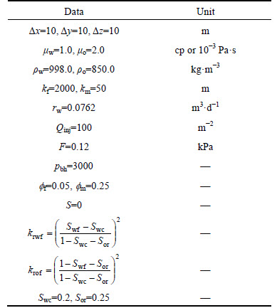
The two-phase flow of oil and water is simulated in a two-dimensional homogeneous reservoir model. The size of reservoir is 300 m×300 m×10 m. In order to evaluate the effectiveness of the streamline simulator, its results are compared with the results of the IMPES technique, and also the results of commercial software of CMG-IMEX [21]. In this reservoir, there is an injection well at bottom-left corner and a production well at top-right corner. Injection well is controlled by water injection rate and the production well is controlled by the bottom-hole pressure. A structured mesh with 30×30×1 grid blocks is generated in order to solve the problem. It is worth mentioning that local timesteps to solve the saturation on streamlines are selected by the CFL criterion [14]. Other properties of the reservoir and the fluid are presented in Table 1.

Table 1 Problem input data

5 Results and discussion

100 streamlines are considered to be traced between the injector and the producer and the total simulation time is 500 d. The pressure will be updated each 100 d and the time steps for solution of the saturation equation on streamlines are calculated based on the Courant– Friedrichs–Lewy (CFL) condition for CFL=0.95.

Figure 1 shows the distribution of time of flight in the first step of the global timestep within the reservoir (the first 100 d of simulation). Using this parameter, we can observe approximate location of front of flow at different moments. For example, the contour line with TOF of 100 d, shows the approximate location of injected water front after 100 d. These results can be compared to the saturation distribution after 100 d. Figure 2 shows the distribution of streamlines traced within the reservoir. As expected, the distribution of streamlines within the reservoir is completely uniform due to the uniform distribution of reservoir permeability and homogeneity. The relationship between wells can be studied well using the distribution of streamlines. The streamlines between two wells show the share of production from the injection rate.

The contours of water saturation distribution in fracture and matrix, after 100, 300 and 500 d are given in Figs. 3 and 4, respectively. In these figures, the results of streamline simulation are compared with those of the IMPES and commercial software. Considering these figures, it can be found that the results are in good agreement with each other. In addition, the difference becomes greater with increasing simulation time. This difference might be caused by the error of frequent mapping between streamlines and the Eulerian grid, which will be increased over the simulation time. Next, we will explain that this difference in the results is in acceptable range. According to the distribution of TOF in Fig. 1, and also based on the water saturation contours in matrix and fracture, which are exhibited in Figs. 3 and 4, respectively, it can be concluded that water progresses symmetrically in the reservoir as a consequence of homogeneous and uniform distribution of the permeability. By approaching the water to the production well, the velocity of the fluid increases and after about 500 d the water reaches to the producer. Some minor differences can be seen in saturation distribution in the vicinity of the wells caused by different well treatment in the two methods. Since in the streamline technique the streamlines are launched from well faces, this is a source of error which makes the results slightly different around the wells.

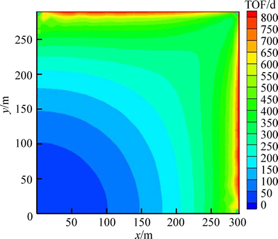
Fig. 1 Contours of time of flight in first global timestep (first 100 d)

Fig. 2 Streamlines in first global timestep (first 100 d of simulation)

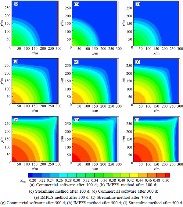
Fig. 3 Water saturation in matrix using different methods:

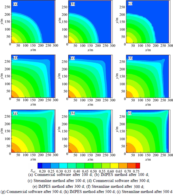
Fig. 4 Water saturation in fracture using different methods:

Comparing Figs. 3 and 4, it can be seen that flow patterns of both streamline and IMPES methods, as well as commercial software are almost coincided. As expected, the flow speed and water saturation in fracture are more than those in matrix, since the permeability of fracture is more than that of matrix.

The results of the volumetric oil production rate and cumulative oil volume for the three methods are compared in Figs. 5 and 6, respectively. The results exhibit a little difference; however, the difference is quite acceptable. As can be seen in Fig. 5, the greatest difference between oil production rates can be observed around 500 d of simulation, but the difference is about 3% which is satisfactory. In Fig. 6, the most difference between results can be seen at the end of simulation, since the difference in production rates is cumulated over the simulation time; but this difference is in an acceptable range and is less than 5%.

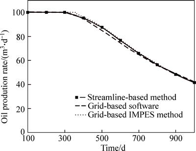
Fig. 5 Comparison of volumetric oil production rates between streamline, IMPES and commercial software during 1000 d of simulation

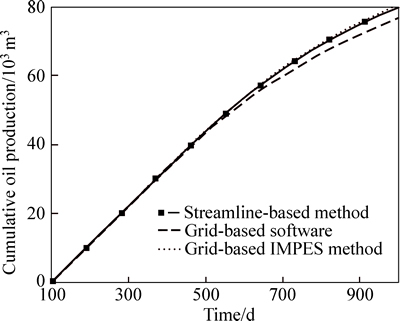
Fig. 6 Comparison of cumulative oil production volume between streamline, IMPES and commercial software during 1000 d of simulation

To investigate the speed of both simulation techniques, the streamline and IMPES codes are run on the same computing systems. The simulation process time for IMPES method lasts 22.3 s; while this time is 3.2 s for the streamline simulator. It is observed that the streamline simulator in this problem can operate up to 7 times faster than IMPES simulation method. Moreover, this time depends on the reservoir size, number of grid blocks, settings of the streamline method and the heterogeneity of the reservoir. However, according to the findings of other researchers [22], the streamline technique is faster than common methods for highly heterogeneous reservoir models with a large number of grid blocks, and increasing the complexity of the reservoir model leads to increased comparative advantage of streamline simulation method.

6 Conclusions

1) Streamline simulation can be a good choice to be used beside conventional reservoir simulators, as a consequence of high-speed computation capability, less required computer memory, proper accuracy and providing good information about flow in the reservoir.

2) In this work, two in-house codes are developed to simulate two-phase flow in naturally fractured reservoirs using the streamline simulation and IMPES methods.

3) The governing equations are presented by the streamline and IMPES methods and then the dual porosity model is employed to model the fractured reservoir.

4) The Kazemi’s transfer function is considered in order to express transfer terms between the fracture and the matrix; the shape factor used in the transfer function is based on the Kazemi’s model.

5) Then, a two-dimensional homogeneous fractured reservoir is defined; the waterflooding process is modeled using both the streamline and IMPES methods and finally the results are compared in terms of water saturation in fracture and matrix, oil production flow rate and cumulative oil production. Comparing these results with those of a commercial software reveals that the streamline simulation can produce proper results with satisfactory accuracy, consuming less times for simulation. Such that the streamline technique in this work is about 7 times faster than the IMPES method.

List of symbols

Permeability, k                   m²

Flow rate, q                      m³

α phase saturation, S_α    Dimensionless

Pressure, p                      kPa

Well index, I_w                        m³

Skin factor, S                    m

Well loop radius, r_w                 m

Equivalent radius, r_e          Dimensionless

α phase flow fraction, f_α        m³

Transfer function, T             m^-2

Form factor, F                  m·s^-1

Darcy velocity, U               m·s^-1

Actual velocity, V              m·s^-1

Maximum saturation change, S_max  Dimensionless             

Time of flight, τ                 s                       

Time of flight to cross the cell, △τ   s

Overall time step, △t_p               s

Porosity factor, f              Dimensionless

Factor mobility, λ              Pa^-1·s^-1

Viscosity, μ                    Pa·s

Subscripts

f                               Fracture

m                               Matrix

w                               Water

o                                Oil

c                              Critical

bh                            Bottom-hole

cm                             Capillary

References

[1] ALIZADEH B, TELMADARREIE A, SHADIZADEH S, TEZHE F. Investigating geochemical characterization of Asmari and Bangestan reservoir oils and the source of H₂S in the Marun oilfield [J]. Petroleum Science and Technology, 2012, 30(10): 967-975.

[2] van GOLF-RACHT T D. Fundamentals of fractured reservoir engineering [M]. New York: Elsevier, 1982.

[3] CHEN Z, HUAN G, MA Y. Computational methods for multiphase flows in porous media [M]. Philadelphia, USA: Society for Industrial and Applied Mathematics, 2006.

[4] DOUGLAS J, HENSLEY J L, ARBOGAST T. A dual-porosity model for waterflooding in naturally fractured reservoirs [J]. Computer Methods in Applied Mechanics and Engineering, 1991, 87(2): 157-174.

[5] THIELE M R, BATYCKY R, IDING M, BLUNT M. Extension of streamline-based dual porosity flow simulation to realistic geology [C]// 9th European Conference on the Mathematics of Oil Recovery. 2004.

[6] BATYCKY R, BLUNT M J, THIELE M R. A 3D field-scale streamline-based reservoir simulator [J]. SPE Reservoir Engineering, 1997, 12(4): 246-254.

[7] TANAKA S, ARIHARA N, AL-MARHOUN M A. Evaluation of oil compressibility effects on pressure maintenance in naturally fractured reservoirs using streamline simulation [C]// International Oil and Gas Conference and Exhibition. China: Society of Petroleum Engineers. Beijing, China. 2010: SPE-131716.

[8] POLLOCK D W. Semianalytical computation of path lines for finite-difference models [J]. Groundwater, 1988, 26(6): 743-750.

[9] GILMAN J R, KAZEMI H. Improvements in simulation of naturally fractured reservoirs [J]. SPE J, 1983, 23(4): 695-707.

[10] DI DONATO G, WENFEN H S, BLUNT M J. Streamline-based dual porosity simulation of fractured reservoirs [C]// SPE Annual Technical Conference and Exhibition. Denver, Colorado, 2003: SPE-84036.

[11] LIM K, AZIZ K. Matrix-fracture transfer shape factors for dual-porosity simulators [J]. Journal of Petroleum Science and Engineering, 1995, 13(3): 169-178.

[12] DI DONATO G, BLUNT M J. Streamline-based dual-porosity simulation of reactive transport and flow in fractured reservoirs [J]. Water Resources Research, 2004, 40(4): W04203.

[13] AL-HUTHALI A, DATTA-GUPTA A. Streamline simulation of counter-current imbibition in naturally fractured reservoirs [J]. Journal of Petroleum Science and Engineering, 2004, 43(3): 271-300.

[14] SIAVASHI M. Thermal enhanced oil recovery modeling in oil reservoirs using streamline simulation [D]. Tehran, Iran: University of Tehran, 2013.

[15] ERTEKIN T, ABOU-KASSEM J H, KING G R. Basic applied reservoir simulation [M]. Texas: Society of Petroleum Engineers Richardson, 2001.

[16] IINO A, ARIHARA N. Use of streamline simulation for waterflood management in naturally fractured reservoirs [C]// International Oil Conference and Exhibition. Mexico: Society of Petroleum Engineers, 2007: SPE-108685.

[17] SIAVASHI M, BLUNT M J, RAISEE M, POURAFSHARY P. Three-dimensional streamline-based simulation of non-isothermal two-phase flow in heterogeneous porous media [J]. Computers & Fluids, 2014, 103: 116-131.

[18] SIAVASHI M, POURAFSHARY P, RAISEE M. Application of space–time conservation element and solution element method in streamline simulation [J]. Journal of Petroleum Science and Engineering, 2012, 96: 58-67.

[19] DI DONATO G, HUANG W, BLUNT M J. Streamline-based dual porosity simulation of fractured reservoirs [C]// SPE Annual Technical Conference and Exhibition. Denver, USA: Society of Petroleum Engineers, 2003: SPE-84036.

[20] CHEN Z. Reservoir simulation: Mathematical techniques in oil recovery [M]. Philadelphia; USA: Society for Industrial and Applied Mathematics, 2007.

[21] Computer Modelling Group. User’s Guide IMEX Advanced Oil/Gas Reservoir Simulator (CMG) [M]. Alberta: University of Calgary, 2004.

[22] SAMIER P, QUETTIER L, THIELE M. Applications of streamline simulations to reservoir studies [C]// SPE Reservoir Simulation Symposium. Society of Petroleum Engineers. Texas. 2001: SPE- 66362.

(Edited by FANG Jing-hua)

Received date: 2015-08-06; Accepted date: 2015-12-10

Corresponding author: Mohammad Hossein Doranehgard; Tel: +98-916-9456250; E-mail: m_doraneh@mecheng.iust.ac.ir