J. Cent. South Univ. (2016) 23: 955-968

DOI: 10.1007/s11771-016-3143-8

Pedestrian environment prediction with different types of on-shore building distribution

SONG Xiao-cheng(宋晓程)¹, LIU Jing(刘京)², YU Lei(余磊)³

1. School of Municipal and Environmental Engineering, Harbin Institute of Technology, Harbin 150090, China;

2. State Key Laboratory of Urban Water Resource and Environment (Harbin Institute of Technology),

Harbin 150090, China;

3. Shenzhen Key Laboratory of Urban Planning and Decision Making (Harbin Institute of Technology),Shenzhen 518055, China

 Central South University Press and Springer-Verlag Berlin Heidelberg 2016

Abstract: The aim of this work is to evaluate how the building distribution influences the cooling effect of water bodies. Different turbulence models, including the S-A, SKE, RNG, Realizable, Low-KE and RSM model, were evaluated, and the CFD results were compared with wind tunnel experiment. The effects of the water body were detected by analyzing the water vapor distribution around it. It is found that the RNG model is the most effective model in terms of accuracy and computational economy. Next, the RNG model was used to simulate four waterfront planning cases to predict the wind, thermal and moisture environment in urban areas around urban water bodies. The results indicate that the building distribution, especially the height of the frontal building, has a larger effect on the water vapor dispersion, and indicate that the column-type distribution has a better performance than the enclosed-type distribution.

Key words: CFD simulation; micro-climate; unban water body; building distribution

1 Introduction

It is well known that the urban air temperatures of most large cities increase gradually in recent years [1-2]. It is also understandable that the concern regarding the methods of improving the quality of the urban thermal environment is increasing dramatically. Meanwhile, there have been many studies focusing on the relationship between the urban thermal environment and the surface-covering conditions [3-7]. The natural underlying surfaces such as water bodies, have the potential to improve pedestrian environment by increasing the surface moisture availability similar to rural areas [8-10].

Compared with many researches on hydraulic characteristics of water bodies, few studies aim at the impact of water bodies on the urban outdoor environment and work on quantifying the cooling effect in vertical and horizontal space [11-12]. The process of restoring a large stretch of inner-city stream in Seoul, Korea, provided the opportunity of demonstrating the cooling effect of the stream on urban microclimate [13]. Studies of different kinds of water bodies in different regions show that the cooling effects in the locality can vary from 0.5 to 5 °C [11, 14]. Further studies show that the cooling effect of water body is connected with not only the hydraulic characteristics but also the weather and season. HATHWAY and SHARPLES [15] found a mean level of daytime cooling of over 1.5 °C above river in spring, but reduced in summer. XU et al [16] analyzed the thermal comfort near water body on hot summer days and proposed an index for evaluating the artificial lake effectiveness. However, most of these researches are limited to field measurements and they can only give the current situations of the certain thermal environment and cannot give the assistance in the planning stage of different districts.

On the other hand, in predicting the outdoor environment in street scale, the pedestrian environment is not only related to land cover, but also affected by various planning factors such as building type and local urban form. Previous study indicated that the architectural layout was an important factor in reducing the urban heat island [17]. Some other researchers also focused on finding out the role of planning factors in pedestrian environment, such as local urban form in wind and thermal environment [18-23]. However, none of them combined those factors with water body. Research on the relationship between multiple morphological characteristics and the ability of propagation of the cooling effect of water body is also limited. Due to the increasing urban development in the waterfront area [24], the demand of this kind of research becomes greater and meaningful recently [25].

For this purpose, we used computational fluid dynamics (CFD) to discuss the pedestrian environment of the residential district around the water and reproduce the whole flow field data in various physical processes as CFD is very suitable for parametric studies. On the other hand, the accuracy of turbulence models in evaluating heat and moisture transfer on a large scale is another concern. Therefore, in this work, CFD simulations were firstly validated by detailed wind tunnel experiments which evaluated the performance of different turbulence models for predicting the water vapor dispersion around building complexes. The method of reproducing the water vapor diffusion in CFD setup was discussed and then the RNG model was used to predict the thermal and moisture environment considering solar radiation and water vapor dispersion at a full scale integrating the theory of urban planning. The effects of important factors on the water vapor dispersion were investigated in the micro- climate around water bodies. We focused on the relevance between the layouts of building blocks and the ability of propagation of the cooling effect, proposing the optimal design for relieving the heat island effect. The influence of those factors on the propagation of the cooling would be beneficial for providing guidance on water body regeneration for an improved microclimate.

2 Methodology

2.1 Models

For most engineering applications, Reynolds Averaged Navier Stokes (RANS) turbulence models can provide fairly accurate solutions for a wide range of air flow problems while requiring relatively low computational resources. The basic principle of the turbulence modeling approach is the application of the Reynolds-averaging operator to the Navier Stokes equations, resulting in the appearance of new unknowns: the Reynolds stresses. These stresses can be linked to the flow variables in different ways, which define the type of turbulence model. Among the different RANS turbulence models, two-equation (2-eq) turbulence models are widely used in predicting the wind environment with actual buildings [26].

Therefore, in this work, various RANS turbulence models including S-A, SKE, RNG, Realizable, Low-KE and RSM are presented for moisture dispersal around water bodies. These models can quickly predict air distributions and in the 1970s, they have been developed for the treatment of eddy viscosity. The Spalart-Allmaras model, known as S-A, with 1-eq, solves the transport equation for eddy viscosity [27]. This model is considered as one of the accurate turbulence models for free shear and boundary layer flows. SKE is the standard k-ε model, which is one of the most prevalent 2-eq models for airflow simulation due to its simple format, robust performance and wide validations [28]. Many attempts have been made to develop 2-eq models that improve on the SKE. RNG is the Re-Normalization Group k-ε model [29]. It was reported that RNG model provides substantially better predictions than SKE for turbulent flow over a backward facing step in separated flows attributed to the better treatment of near wall turbulence effects [30]. Another high Reynolds number k-ε model is Realizable (realizable k-ε) model [31]. Realizable models usually provide much improved results for swirling flows and flows involving separation when being compared to the SKE. Previous research indicated the Realizable k-ε model performs better than the SKE for predicting various buoyancy plumes [32]. The Low-KE model is the low-Reynolds-number k-ε model. It is an improved k-ε model and is usually used to connect the outer-wall free stream and the near-wall flow. This model overcomes the disadvantages of SKE in predicting low Reynolds number flows [33]. RSM (the Reynolds stress model), instead of calculating the turbulent eddy viscosity, explicitly solves the transport equation of Reynolds stresses and fluxes [34]. Previous research has shown that RSM is superior to the SKE model because anisotropic effects of turbulence are considered [35].

The interaction between water body and air is one of the main issues when dealing with water vapor dispersion. Theoretically, the water vapor diffusion should be coupled with the heat transfer at water surface. However, it is difficult for a large scale and unstable simulation by the existing CFD technologies. Previous studies firstly simplified this problem to how to deal with the water surface temperature. They discussed the dynamic or spatial variation of water surface temperatures under different conditions [36-39]. Some of them indicated that the temperature variation of water body in a short period (several hours or a day) is very small and could be neglected when being compared with long- term variation [40]. Therefore, in this work, it is reasonable to conduct a steady simulation without considering the dynamic change of water surface temperature for time saving. The interaction between the fluid (air) and the water vapor is treated as one-way coupling, assuming that the effect of water vapor on the turbulent flow is negligible due to the low water vapor loadings. The water vapor diffusion between water surface and atmosphere is another important issue. Previous researchers widely used bulk method to simplify the complex heat exchange between water body and air. The general form of evaporation is written as follows [41]:

                         (1)

where E_v is the evaporation rate at the water/air interface, mm/s; U is the wind velocity at a certain height above the water body, m/s; E_w is the specific humidity of air close to the water surface, kg/kg; C_t is the empirical coefficient and related to the wind velocity and atmospheric stability [41]; E_a is the specific humidity of air, kg/kg; ρ_a is the air density, kg/m³.

Solar radiation is one of the main processes during outdoor pedestrian environment simulation. The solar ray tracing model, which works as the source of the solar heat in the energy equations, was employed when analyzing the water vapor evaporation in the urban waterfront cases.

2.2 Model verification

2.2.1 Brief introduction to wind tunnel experiment

The wind tunnel experiment was performed by NARITA [42]. The outline of the wind tunnel workstation is shown in Fig. 1. The test section of the wind tunnel was located in a backflow area. The size of the in-vent was 0.9 m high and 1.8 m wide. All of the blocks had the same size and were distributed uniformly. The size of the cubic block was 0.03 m. The blockage ratio was 0.5%. The dimension of water body model was 0.2 m (width), and 2 m (length), along with blocks. Considering the embankment effect, the height between water surface and ground was approximately 0.005 m. The measurement instruments for the temperature and humidity were a 0.1 mm thermocouple with an accuracy of 0.01 °C and a capacity-type hygrometer with an accuracy of 5%.

The wind direction, water body and relative position of the buildings are shown in Fig. 2. The sampling points, as given in Fig. 1, was 0.01 m high (measured from the ground) and 1.75 m from the reference point. The reference point shown in Fig. 1 was at the left edge of the water channel. The mean velocity profile within the neutral ABL (atmospheric boundary layer) was given by the exponential distribution:

                             (2)

where the power-law exponent α is equal to 0.25, according to the wind tunnel experiment; u(z₁)=3 m/s, which is the mean wind velocity at the reference height z₁ of 0.3 m; z is the height above the ground.

The measured streamwise turbulent intensity was 20% at the top level of the blocks, and the block boundary layer thickness was approximately 0.3 m. The water temperature was set slightly higher than ambient air temperature.

2.2.2 Domain and grid

According to the setup in the wind tunnel experiment, the computational domain size was set as 3200 mm×2000 mm×305 mm, i.e. 106H_b, 66H_b and 10H_b (H_b is the height of the cube), which reproduces the actual wind tunnel condition. The length and width of the block area were approximately 1970 mm and 390 mm, respectively. The distance from the first row to the embankment was set at 10 mm.

To guarantee good accuracy and convergence stability, six turbulence models, the S-A, SKE, RNG, Realizable, Low-KE, and RSM models, were discussed  with changing the mesh of the structured grid to realize high possible grid resolution according to the computer ability. Low-KE model has higher sensitivity in the range near the wall surface compared with other 2-eq models in the study. Thus, Low-KE model was employed to test the grid independence in the study. Four cases with different grids were investigated, i.e. 1.8×10⁶ cells, 2.6×10⁶ cells, 3.3×10⁶ cells and 4×10⁶ cells. The results indicated that for Low-KE model, the difference of mass fraction of water vapor between the case with 4×10⁶ cells and the case with 3.3×10⁶ cells is very small. Thus, 3.3×10⁶ cells were employed in the numerical simulation in the study.

Fig. 1 Workstation in wind tunnel (Unit: mm)

Fig. 2 Distribution of blocks (Unit: mm) [42]

The computational domain was compartmentalized into approximately 2.3×10⁶ structured grids and the Y⁺ of the first grid above water surface was about 10 when using the S-A and SKE models. However, for the Low- KE and RSM models, the grids were increased to approximately 3.3×10⁶ with extra grids close to the water surface. To obtain the performance of the linear layer above the water surface, Y⁺ of the first grid above water surface was confirmed at approximately 3 after thinning the grid. Figure 3 shows the grid conditions used for the Low-KE model as an example.

2.2.3 Calculation conditions

The setup of wind tunnel experiments was completely reproduced in the CFD simulation. Since no solar radiation occurred during the wind tunnel measurement, solar radiation model was not included when validating the water vapor evaporation with the wind tunnel measurement. For all of the RANS models, the basic equation used in this work was the steady, incompressible, three-dimensional Reynolds- averaged Navier-Stokes equation. At the inflow boundary, a velocity profile for the atmospheric boundary layer was applied. The velocity profile was constructed using   Eq. (1). The turbulent intensity of the S-A model was the measured data in the wind tunnel experiment, and the turbulent length scale was set at 30 mm according to the characteristic length. For the 2-eq RANS models and the RSM model, both the kinetic energy and dissipation rate should be considered. The linear pressure-strain RSM model was used and the near-wall treatment was enhanced wall treatment. The vertical profiles of these turbulent parameters were constructed as follows [26]:

                       (3)

                           (4)

                         (5)

where I(z) is the turbulent intensity at the height z, %; k(z) is the turbulent kinetic energy at the height z, m²/s²; ε(z) is the turbulent dissipation rate at the height z, m²/s³; z_G is the boundary layer thickness of 0.3 m; α is equal to 0.25, according to the wind tunnel experiment; C_μ is constant to be 0.09.

Fig. 3 An example of setup of mesh for Low-KE model

At the lateral surfaces of the computational domain, the conditions of the wall function method were used. At the block surfaces and ground surface, the wall function method of the logarithmic laws was used. At the outflow boundary, the zero gradient conditions were used. All of the transport equations were compartmentalized using the QUICK scheme and SIMPLE algorithm for pressure-velocity coupling.

The empirical coefficient C_t in Eq. (1) is related to wind velocity. According to Ref. [41], C_t could be set as a constant value of 0.00115 when wind velocity was less than 5 m/s, which is just in the range of wind velocity in this CFD simulation. By pre-calculation, the temperature of the water surface was fixed to be 30 °C. The corresponding mass fraction of the vapor at the height of 0.001 m above water surface was estimated to be 0.0269 and then imposed at the water body surface for the water vapor dispersion. Additionally, the temperature of inlet air was fixed to be 27 °C and the mass fraction of the water vapor was imposed at inlet for 0.0181. The species transfer model was applied to predict the diffusion of water vapor in whole region. The commercial software Fluent 6.3 was used for all of the calculations.

2.2.4 Validation

Numerical simulation on water vapor diffusion was validated through a comparison of measured data from Narita 1992. Due to the lack of measured temperature and wind flow distribution, those corresponding values in the CFD simulation were not validated in this work.

Figure 4 shows the distribution of the water vapor mass fraction at the section of the sampling area calculated by each turbulence model. Meanwhile, the detailed distribution of the water vapor mass fraction near the embankment is shown on the upper-left of each turbulence model. As can be seen from the detailed figures, the water vapor mass fraction in all models has layered distribution and decreases with height increasing. At the height of the ground, the SKE model and the RNG model apparently show a lower value than other models. From the general figures, it is obvious that each figure compares different results of the water vapor distribution with each other, especially at the scale of dispersion above the water body and in the sampling area. Compared with other models, the result calculated by RSM model seems to have a higher level of water vapor in the sampling area. The distance of dispersion on each side of the embankment is much longer, and the mass fraction of water vapor above the water surface and in the adjacent area is higher than that calculated by 2-eq models. The 2-eq models have almost the same dispersion scale above the water surface and surroundingspace. It is clear that the S-A model has a larger fluctuation with a higher value of the water vapor mass fraction above the water and a lower value in the sampling area.

There are several parameters that are used for verification. The humidity ratio is defined as follows:

                                     (6)

where m_v is the water vapor mass of wet air, kg; m_a is the water vapor mass of dry air, kg.

The mass fraction of the water vapor is defined as follows:

                                (7)

Combining Eqs. (6) and (7), we obtain the following equation:

                                   (8)

From the above equations, we can see that the mass fraction of the water vapor is larger when the airflow tends toward saturation.

To obtain the characteristic water vapor dispersion within the blocks around the water, the wind tunnel results consider the vapor pressure ratio VP (R) as an evaluation index of the diffusion effect, which is defined

Fig. 4 Distribution of water vapor mass fraction at section of sampling area:

as

                         (9)

where e is the vapor pressure at the sampling point, Pa; e₀ is the vapor pressure at the reference point, Pa; e_s is the saturated vapor pressure related to the water surface temperature, Pa.

Figure 5 shows the comparison between different turbulence models and wind tunnel experimental results. The measurement data change dramatically when the distance increases. The VP begins at approximately 0.12 and increases to the peak level of 0.15 above the embankment. Then, the value decreases sharply to approximately 0.05 when Y/W increases to approximately 0.75 and then decreases slowly with increasing the distance. The simulation results by the six turbulence models show a similar trend except for those in the S-A model. However, all of the predicted VP values above the water body are higher than the experimental results and lower in the sampling area. This trend becomes more obvious with increasing distance ratio Y/W. The results could be due to several reasons. First, the water vapor of the water surface is set up based on the saturated humidity ratio, which is a function of the water temperature. This value might be set slightly higher than the actual situation because of the lack of accurate measurement data of temperature, which leads to a higher prediction in the water vapor dispersion. Secondly, the 2-eq turbulence models have some disadvantages in solving the airflow around buildings, leading to a lower prediction around buildings. Thirdly, the dynamic characteristic of the wind tunnel is not reported, along with the turbulence in three dimensions, uniformity and airflow conditions in wind tunnels. Overall, all RANS models, especially 2-eq models, are suitable for solving thermal and water vapor dispersion problems under the conditions in the study.

To compare the performance of various turbulence models, the index of the average relative error of VP values (AREVP) was introduced in this study, which is given by

                    (10)

where R_s is the simulated VP values at the sampling points; R_m is the measured VP values at the sampling points; n is the number of the sampling points.

Table 1 shows the AREVP of the different turbulence models. It is apparent that the VP values are smaller than 0.03 when Y/W is higher than 1.0 (Fig. 5), i.e. boundary of the second array. Considering that the values might be affected by the instrument precision, the VP values are not analyzed as a main concern when Y/W is higher than 1.0 in this work. It can be seen that the error of RNG model is apparently lower than that of other models in the area above river, which demonstrates that RNG model is effective for this kind of airflow. For the areas at first two arrays and behind first two arrays, RSM model performs better than other models. That is possibly because RSM model has been considered to be accurate when analyzing flow with strong anisotropic behaviors around building blocks with increasing complexity. However, RSM model seems to fail in predicting the airflow above river. That is because many more assumptions and modeling of various terms in the Reynolds stress transport equation weaken the simulation accuracy instead. Some studies found that the RSM model was not improved in many results in predicting a simple airflow such as natural convection [43]. Based on simulation results, the Low-KE model is expected to have a relatively better performance than the SKE model, especially for handling near-wall flows, which is in accordance to turbulence theory [44]. The simulation results of RNG model have the best overall performance in the whole areas in terms of accuracy, numerical stability, and computing time attributed to improved effective viscosity prediction and better treatment of near wall turbulence effects, while RSM model also has the competitive performance.

Fig. 5 Simulation results of different turbulence models vs measured results

Table 1 Average VP relative errors of different turbulence models

3 Model procedure

3.1 Simulation uncertainty analysis

The uncertainty of outdoor thermal environmental simulation may arise from a variety of sources. In this work, two general sources contributed to the uncertainties in simulation predictions: the internal uncertainty and the external uncertainty [45]. The internal uncertainty includes the uncertainty in the validity of the assumptions underlying a specific model. This is mainly due to the limited information in selecting and estimating the characteristics of the model parameters. In this work, several turbulence models were compared with wind tunnel experiments, which were discussed above, to select the most suitable model for prediction. The purpose of this analysis is to minimize the internal uncertainty to the large extent. On the other hand, the external uncertainty came from the variability in model prediction arising from plausible alternatives for input values. In this work, this type of uncertainty mainly includes the variabilities associated with meteorology and underlying surfaces. From a practical perspective, the complexity of outdoor thermal environmental simulation is within the limitations on computer ability and time consuming. The real conditions of water body and building distribution in waterfront are too complicated to be modeled, such as thermophysical property and form, so dose the combination of variable underlying surfaces. Therefore, due to the complexity, we emphasized the predominant underlying surfaces and idealized the building type in a reasonable way, which has notably thermal effect. Although proper assumptions and simplifications were used in this work, the input parameters were well founded on the guidelines for outdoor environment prediction [26]. The meteorological input used standard summer design values in Harbin after statistics [46]. Other inputs such as thermophysical property used routine values under the condition of Harbin.

3.2 Physical models

In this work, the RNG model was used to predict the moisture distributions because the results from this model showed a relatively good agreement with the wind tunnel results mentioned above. Various building distributions in urban waterfronts can be found in China, as shown in Fig. 6. In this work, four types of waterfront plans were considered (as shown in Fig. 7). These waterfront plans can be considered to represent the actual distributions of building complexes in the northern cities of China. The characteristic climate in northern China is hot in the summer and very cold in the winter, therefore, the orientation of the buildings is mostly toward south to gain more sunshine. Additionally, a number of factors were considered, such as layouts of building complexes, including different building shapes, heights, and number of rows. Case A is a column type that represents the high-rise commercial or residential buildings that are mainly built along the water body. Case B is a board-style construction of multi-storey buildings and is a column type. This type indicates that this waterfront area is mainly mixed with residential and small-scale business buildings. A local enclosed type was adopted in Case C and Case D with different building floor area ratios. It should be noted that the local enclosed type is very popular in northern China because this type can be considered to block more cold airflow into the internal area in winter. The detailed information about each case is summarized in Table 2.

3.3 Simulation conditions

To simplify the simulation, the water body was set up as straightforward with an east-west direction. Thewidth of the water body in every case was considered to be 150 m, which can be considered as a medium urban river in northern China. Additionally, the distance from the first row of buildings to the embankment was 120 m. To obtain a regularity of the thermal climate affected only by the distribution of buildings to the large extent, all of the underlying surfaces were set as artificial impervious surfaces except for the water surface, and the vegetation was not considered in this work.

Fig. 6 Actual layouts of building complex along water body in a northern city of China:

Fig. 7 Four types of building layouts on waterfront:

Table 2 Detailed information of each building layout

The boundary conditions were set based on the field measurement data in previous studies [47] and are summarized in Table 3.

At the lateral and upper surfaces of the computational domain, the symmetry conditions were used, where the normal velocity component and normal gradients of the tangential velocity components were set to be zero. At the building surfaces and ground surface, the wall functions based on the logarithmic laws were used. The thermal conductivity was 1.5 W/(m·K), and the heat transfer coefficient was set to be 23 W/(m²·K). The external emissivity of the building array was 0.9. The buildings and ground absorption of direct visibility were 0.2 and 0.9 of the direct infrared radiation (IR), respectively [49]. At the outflow boundary, zero gradient conditions were used. All of the transport equations were compartmentalized using QUICK scheme, and SIMPLE algorithm was used for pressure-velocity coupling.

Table 3 Main boundary conditions

To investigate the sensitivity of the grid resolution, each case was first compartmentalized to a lower grid resolution (approximately 0.7×10⁶ cells), medium grid resolution (approximately 1.5×10⁶ and 2.4×10⁶ cells) and higher grid resolution (approximately 3.6×10⁶ cells). As shown in Fig. 8, little difference of both mass fraction and temperature results among 1.5×10⁶, 2.4×10⁶ and 3.6×10⁶ grids was observed during the grid independence test. Employing 1.5×10⁶ grids could not only guarantee the simulation precision but also enhance the computer efficiency.

Fig. 8 Grid independence test results of Case B:

Compared with the others, the medium grid resolution showed enough calculation accuracy and an appropriate calculation time. Therefore, in each case, the grid adopted the medium resolution, and the dimensions of the domain were 15H_b, 18.5H_b, and 7H_b (H_b is the maximum height of cube) in the x, y, and z directions, in line with the AIJ guidelines for the practical application of CFD to pedestrian wind environments around the buildings. An upstream distance of 5.5H_b with the origin of the coordinate system at the first line of the cube was considered according to the AIJ guidelines. The grid near the wall and the water body was adjusted for good accuracy. The minimum grid width was 0.3 m and Y⁺ of the first grid near the wall was confirmed at approximately 60 after thinning the grid. Figure 9 shows the mesh of Case B as an example.

Fig. 9 Simulation domain and mesh of Case B:

3.4 Evaluation indices and sampling points

To discuss the relevance between the building layouts and water vapor dispersion, two non-dimensional indices were proposed to evaluate the thermal environments of different cases in this work. The air temperature and humidity were used as indicators to evaluate the thermal environments. These non- dimensional indices had the advantage of eliminating the uncertainty caused by different cases. The expressions were defined as follows:

                         (11)

                     (12)

where t_v is the temperature at the sampling point, °C; t₀ is the temperature at the water surface, °C; t_b is the mean air temperature of airflow at the base line, which is assumed to be unaffected by the water body, °C; m_v is the mass fraction of water vapor at the measuring point; m₀ is the mass fraction of the water vapor at the water surface; m_b is the mean mass fraction of the water vapor of airflow at the base line, which is upwind of the water body assumed to be unaffected by water.

To analyze the effect of water, we selected 11 sections starting from the river center to the edge of the building area (Fig. 10). As observed from the wind tunnel experiment results, the variation of indices became dramatically near to the water body. Therefore, the distance between two sampling sections was set gradually longer when they were away from the water body. The wind direction and details of the location of the base line are also marked in Fig. 11.

4 Results and discussion

4.1 Distribution of thermal environment (Case B)

As an example, Fig. 11 shows the temperature distribution in the intermediate section of Case B (Fig. 10 (b)). It can be observed that due to solar radiation, the temperatures of the building roofs, external walls and grounds, which are exposed to direct sunlight, exceed approximately 45 °C. However, the air around the water body has a lower temperature of approximately 27-30 °C. The reason is that the water body has a lower and more stable temperature during heat storage, advection and latent heat exchange. However, the temperature-affected area by the water is mainly limited to areas above the water body, which indicates that the cooling air cannot transfer to the adjacent building area as expected.

Figure 12 shows the flow vector and water vapor mass fraction in the intermediate section of Case B (Fig. 10 (b)). Different from the temperature distribution, which was affected by various factors such as solar radiation, heat storage and convection by underlying surface, the water vapor distribution was strongly determined by the wind flow. The maximum moisture is at the water surface with a value of 0.022, 0.008 higher than the value at an inlet without any hindrance. Under the influence of the dominant wind, the water vapor flows over the low building near the water body (at a height of 20 m) to the downwind area, and then blocked by high buildings, which indicates that the building height and width near the water body greatly impact the moisture diffusion.

Fig. 10 Positions of sampling points (└ ┘shows location of section):

Fig. 11 Temperature distribution in a longitudinal section of sampling area in Case B (K)

Fig. 12 Vector (a) and water vapor mass fraction (b) in a longitudinal section of sampling area in Case B

4.2 Effect of building floor area ratio on thermal environment (Case B)

In order to quantitatively analyze the effect of building floor area ratio on the thermal environment, cases were discussed based on condition of Case B with different building floor area ratios only. The increase in building floor area ratio presented the building height increase as we fixed the building type as column-type and the board style construction. We used the surface average values of the whole building area at the height of 1.5 m as the evaluation index. The specific conditions are given in Table 4.

Figure 13 shows the effect of building floor area ratio on water vapor mass fraction and temperature. The m_v and t_v were calculated by the surface average value of the whole building area. The building floor area ratio showed an obvious linear effect on mass fraction ratio of the water vapor. The m_v decreased by 27.6% when the building floor area ratio increased from 0.5 to 5.0. This attributes to lower wind velocity caused by the higher building floor area ratio. On the other hand, the effect of building floor area ratio on temperature was much more complicated. The t_v showed an uptrend when the building floor area ratio increased from 0.5 to 2.0 and from 3.5 to 5.0, then went down when building floor area ratio increased from 2.0 to 3.5. The reason for this trend is that the higher building floor area ratio affects not only the wind environment but also the sunshade. The results indicated an integrated effect on the thermal environment.

Table 4 Orthogonal experiment design

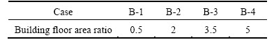
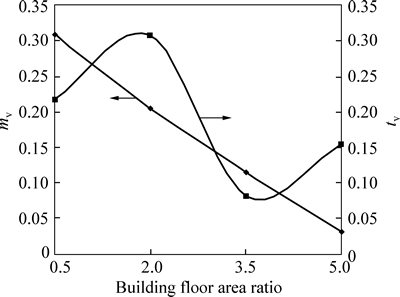
Fig. 13 Effect of building floor area ratio on water vapor mass fraction and temperature

4.3 Effect of building type on thermal environment

Figure 14 shows the distribution of t_v of the four cases. Y represents distance from the center of the water body, and W represents the width of the water body. In this work, t_v was calculated as the spatial-average value at a height of 1.5 m from the ground in the sampling sections, which are shown in Fig. 10. It can be observed that most of the cases remain at the same with lower temperature above the water body and higher temperature in the building area. The values in every case begin at the low level of 0.03 and stay the same above the water body due to the cooling effect of the water body itself. Then, these values increase rapidly when the sampling points are located away from the water surface. The main reason for this increase is that air is heated by convection at the ground due to solar radiation. After air flows inside the building area, the results have different trend due to the complicated building distribution in each case. It is obvious that t_v values of Case B and Case D are lower than those of the other two cases, meaning that relatively cooler airflow can easily enter the building area. It can be seen from Table 2 that Case B and Case D have a lower height of the frontal buildings. Additionally, Case B and Case D have more building rows, which means more sun shadow at noon at a pedestrian height. This additional shadow is also an advantage of the cooling effect. In contrast, Case A and Case C have both a high building floor area ratio and fewer building rows, leading to more heat gain. However, this heat gain indicates that the cooling effect of the water body does not go far into the building area but is only limited to the neighborhood, and its cooling effect is closely connected to the building distribution.

Fig. 14 t_v vs Y/W of four cases

Figure 15 shows the distribution of m_v of the four cases. First, each case shows a similar trend, and all of the peaks appear at the center of the water body. The m_v decreases dramatically with increasing distance until the airflow reaches the building blocks. Similar to the temperature distribution, the results from Case B and Case D obviously show better performance than the results of Case A and Case C. The values in the former cases decrease slower than those of the latter. As mentioned above, in addition to the concentration difference, water vapor is mainly driven by wind flow, indicating that cooler airflow can flow more easily in Case B and Case D. In contrast, the worst performance appears in Case C, of which the buildings shape is of column-type and enclosed-type, and the building height is large, which leads to mass blocking for water vapor dispersion. However, Case A shows a better performance than Case C, even with a higher building floor area ratio, which indicates that the column type distribution has a better effect on the water vapor dispersion than the enclosed type.

Fig. 15 m_v vs Y/W of four cases

5 Conclusions

1) According to the above discussion, all of the RANS turbulence models agree with the experimental data predicted around the water body to some extent. Compared with the other models, the results calculated by the RSM model have a higher level of water vapor in the sampling area. The two-equation turbulence models have almost same dispersion scale above the water surface and surrounding space. The S-A model shows the worst prediction performance on the water vapor dispersion in the entire area. Although all of the predicted values are greater than the experimental results above the water body, while lower in sampling area, all of the RANS models, especially 2-eq model, are suitable for solving thermal and water vapor dispersion problems under the conditions. RNG model has the best overall performance in the whole areas, while RSM model has competitive performance.

2) It is obvious that the layout of the building groups significantly affects the distribution of the temperature and water vapor. The prediction shows that the cooling effect of the water body decreases with building height. Additionally, the spread length of the water vapor obviously is shortened by the frontal tall building, leading to mass blocking for water vapor dispersion. For the column-type and the board style construction, the water vapor linearly decreases with the building height increasing. While the temperature shows an up-and-down trend with the building height increasing. Additionally, the distributions with more building rows have the advantage of the cooling effect due to more sun shadow at noon at a pedestrian height. This indicates that the building distribution, especially the height of the frontal building, shows a larger effect on the water vapor dispersion and indicates that the column type distribution has better performance than the enclosed type.

3) Due to the complexity of factors influencing the water vapor diffusion near the river, conclusions might be limited to the specific cases discussed in this work. There are still many outdoor factors that we did not consider. A series of quantitative factors selection and evaluation on the water vapor diffusion among the tested configurations should be performed in our future research. More factors and levels, such as vegetation, embankment height, and other building types, should be analyzed combining additional factors of the thermal environment to obtain a complete evaluation of the cooling effect of the water body in different building areas in future studies.

References

[1] ARNFIELD A J. Two decades of urban climate research: A review of turbulence, exchanges of energy and water, and the urban heat island [J]. International Journal of Climatology, 2003, 23(1): 1-26.

[2] TRAN H, UCHIHAMA D, OCHI S, YASUOKA Y. Assessment with satellite data of the urban heat island effects in Asian mega cities [J]. International Journal of Applied Earth Observation and Geoinformation, 2006, 8(1): 34-48.

[3] van GRIEND A A, OWE M. On the relationship between thermal emissivity and the normalized difference vegetation Index for natural surfaces [J]. International Journal of Remote Sensing, 1993, 14(6): 1119-1131.

[4] MARLAND G, SR R A P, APPS M, AVISSAR R, BETTS R A, DAVIS K J, FRUMHOFF P C, JACKSON S T, JOYCE L A, KAUPPI P, KATZENBERGER J, MACDICKEN K G, NEILSON R P, NILES G O, NIYOGI D D S, NORBY R J, PENA N, SAMPSON N, XUE Y K. The climatic impacts of land surface change and carbon management, and the implications for climate- change mitigation policy [J]. Climate Policy, 2003, 3: 149-157.

[5] FEDDEMA J J, OLESON K W, BONAN G B, MEARNS L O, BUJA L E, MEEHL G A, WASHINGTON W M. The importance of land-cover change in simulating future climates [J]. Science, 2005, 310(5754): 1674-1678.

[6] BONAN G B. Forests and climate change: Forcings, feedbacks, and the climate benefits of forests [J]. Science, 2008, 320(5882): 1444- 1449.

[7] KLOK L, ZWART S, VERHAGEN H, MAURI E. The surface heat island of Rotterdam and its relationship with urban surface characteristics [J]. Resources, Conservation and Recycling, 2012, 64: 23-29.

[8] JAUREGUI E. Effect of revegetation and new artificial water bodies on the climate of northeast Mexico City [J]. Energy and Buildings, 1990, 15(3): 447-455.

[9] NISHIMURA N, NOMURA T, LYOTA H, KIMOTO S. Novel water facilities for creation of comfortable urban micro-meteorology [J]. Solar Energy, 1998, 64(4/5/6): 197-207.

[10] PARKER G, SHIMIZU Y, WILKERSON G V, EKE E C, ABAD J D, LAUER J W, PAOLA G, DIETRICH W E, VOLLER V R. A new framework for modeling the migration of meandering rivers [J]. Earth Surface Processes and Landforms, 2011, 36(1): 70-86.

[11] MURAKAWA S, SEKINE T, NARITA K, NISHINA D. Study of the effects of a river on the thermal environment in an urban area [J]. Energy and Buildings, 1990, 16(3/4): 993-1001.

[12] NAGARAJAN B, YAU M K, SCHUEPP P H. The effects of small water bodies on the atmospheric heat and water budgets over the MacKenzie River Basin [J]. Hydrological Processes, 2004, 18(5): 913-938.

[13] KIM Y H, RYOO S B, BAIK J J, PARK I S, KOO H J, NAM J C. Does the restoration of an inner-city stream in Seoul affect local thermal environment? [J]. Theoretical and Applied Climatology, 2008, 92(3/4): 238-248.

[14] LI Shu-yan, XUAN Chun-yi, LI wei, CHEN Hong-bin. Analysis of microclimate effects of water body in a city [J]. Chinese Journal of Atmospheric Sciences, 2008, 32(3): 552-560. (in Chinese)

[15] HATHWAY E A, SHARPLE S. The interaction of river and urban form in mitigating the Urban Heat Island effect: A UK case study [J]. Building and Environment, 2012, 58: 14-22.

[16] XU Jing-cheng, WEI Qiao-ling, HUANG Xiang-feng, LI Guang-ming. Evaluation of human thermal comfort near urban waterbody during summer [J]. Building and Environment, 2009, 45(4): 1072-1080.

[17] ASHIE Y, KONO T. Environmental change due to the redevelopment in Shiodome area [J]. Wind Engineering JAWE, 2006, 31(2): 115-120. (in Japanese)

[18] HE P, KATAYAMA T, HAYASHI T, TSUTSUMI J I, TANIMOTO J, HOSOOKA I. Numerical simulation of air flow in an urban area with regularly aligned blocks [J]. Journal of Wind Engineering and Industrial Aerodynamics, 1997, 67/68: 281-291.

[19] CHEN Hong, OOKA R, HARAYAMA K, KATO S, LI Xiao-feng. Study on outdoor thermal environment of apartment block in Shenzhen, China with coupled simulation of convection, radiation and conduction [J]. Energy and Buildings, 2004, 36(12): 1247-1258.

[20] COIRIER W J, FRICKER D M, FURMACZYK M, KIM S. A computational fluid dynamics approach for urban area transport and dispersion modeling [J]. Environmental Fluid Mechanics, 2005, 5(5): 443-479.

[21] MURAKAMI S. Environmental design of outdoor climate based on CFD [J]. Fluid Dynamics Research, 2006, 38(2/3): 108-126.

[22] CHEN Li. Numerical modeling for the building performance of city underlying surface and thermal environments in Wuhan [D]. Wuhan: Huazhong University of Science and Technology, 2007. (in Chinese).

[23] MOCHIDA A, LUN I Y F. Prediction of wind environment and thermal comfort at pedestrian level in urban area [J]. Journal of Wind Engineering and Industrial Aerodynamic, 2008, 96(10/11): 1498- 1527.

[24] ENDO M. Rapid transit and related urban development in Tokyo waterfront area [J]. Japan Railway & Transport Review, 2005, 42: 38-42.

[25] SHA Yong-Jie, WU Jiang, YAN Ji, CHAN S L T, WEI Q. Xuhui waterfront area: Urban restructuring for quality waterfront working and living, shanghai urbanism at the medium scale [M]. Berlin: Springer Geography, 2014.

[26] TOMINAGA Y, MOCHIDA A, YOSHIE R KATAOKA H, NOZU T, YOSHIKAWA M, SHIRASAWA T. AIJ guidelines for practical applications of CFD to pedestrian wind environment around buildings [J]. Journal of Wind Engineering and Industrial Aerodynamics, 2008, 96(10/11): 1749-1761.

[27] SPALART P, ALLMARAS S. A one-equation turbulence model for aerodynamic flows [C]// Proceedings of the 30th Aerospace Sciences Meeting and Exhibit. Reno, AIAA, 1992: 439-460.

[28] LAUNDER B E, SHARMA B I. Application of the energy- dissipation model of turbulence to the calculation of flow near a spinning disc [J]. Letters in Heat and Mass Transfer, 1974, 1(2): 131-137.

[29] YAKHOT V, ORSZAG S A. Renormalization group analysis of turbulence: Basic theory [J]. Journal of Scientific Computing, 1986, 1(1): 3-51.

[30] SPEZIALE C G, THANGAM S. Analysis of an RNG based turbulence model for separated flows [J]. International Journal of Engineering Science, 1992, 30(10): 1379-1388.

[31] SHIH T H, LIOU W W, SHABBIR A, YANG Zhi-gang, ZHU Jiang. A new k-ε eddy viscosity model for high Reynolds number turbulent flows [J]. Journal Computer Fluids, 1995, 24(3): 227-238.

[32] van MAELE K, MERCI B. Application of two buoyancy-modified k-ε turbulence models to different types of buoyant plumes [J]. Fire Safety Journal, 2006, 41(2): 122-138.

[33] LAUNDER B E, SPALDING D B. The numerical computation of turbulent flows [J]. Computer Methods in Applied Mechanics and Engineering, 1974, 3(2): 269-289.

[34] LAUNDER B E, REECE G J, RODI W. Progress in the development of Reynolds stress turbulence closure [J]. Journal of Fluid Mechanics, 1975, 68(4): 537-566.

[35] MURAKAMIA S, MOCHIDA A, HAYASHI Y, SAKAMOTO S. Numerical study on velocity-pressure field and wind forces for bluff bodies by k-ε, ASM and LES [J]. Journal of Wind Engineering and Industrial Aerodynamics, 1992, 44(1-3): 2841-2852.

[36] EVANS E C, MCGREGOR G R, PETTS G E. River energy budgets with special reference to river bed processes [J]. Hydrological Processes, 1998, 12(4): 575-595.

[37] MASUDA Y, IKEDA N, SENO T, TAKAHASHI N, OJIMA T. A basic study on utilization of the cooling effect of sea breeze in waterfront areas along Tokyo bay [J]. Journal of Asian Architecture and Building Engineering, 2005, 4: 483-487.

[38] MOMII K, ITO Y. Heat budget estimates for Lake Ikeda, Japan [J]. Journal of Hydrology, 2008, 361(3/4): 362-370.

[39] AHMAD S, HASHIM N M, JANI Y M, ALI N. The impacts of sea breeze on urban thermal environment in tropical coastal area [J]. Advances in Natural and Applied Sciences, 2012, 6(1): 71-78.

[40] MOHSENI O, STEFAN H G. Stream temperature/air temperature relationship: A physical interpretation [J]. Journal of Hydrology, 1999, 218(3/4): 128-141.

[41] KONDO J. Transfer coefficients of water surface [J]. Hydrology and Water Resources, 1992, 5: 50-55. (in Japanese).

[42] NARITA K I. Effects of river on urban thermal environment dependent on the types of on-shore building distribution [J]. Journal of Architecture, Planning and Environmental Engineering, 1992, 442: 27-35. (in Japanese)

[43] LEONG W H. Effectiveness of several turbulence models in natural convection [J]. International Journal of Numerical Methods for Heat and Fluid Flow, 1991, 14(5): 633-648.

[44] HSIEH K J, LIEN F S. Numerical modeling of buoyancy-driven turbulent flows in enclosures [J]. International Journal of Heat and Fluid Flow, 2004, 25(4): 659-670.

[45] MALKAWI M A, AUGENBROE G. Advanced building simulation [M]. New York: Spon Press, 2004: 25-29.

[46] China Meteorological Information Center, Department of Building Science of Tsinghua University. Special meteorological data set for building thermal environment analysis in China [M]. Beijing: China Architecture and Building Press, 2005: 121-124 . (in Chinese)

[47] SONG Xiao-cheng, LIU Jing, GUO Liang. Field measurement of the large urban river effect on urban thermal climate [C]// Proceedings of 2011 International Conference on Computer Distributed Control and Intelligent Environmental Monitoring. Changsha, 2011: 71-74.

[48] RICHARDS P J, HOXEY R P. Appropriate boundary conditions for computational wind engineering models using the k-ε turbulence model [J]. Journal of Wind Engineering and Industrial Aerodynamics, 1993, 46-47: 145-153.

[49] BRUSTSAERT W. Evaporation into the atmosphere: Theory, history, and applications [M]. Dordrecht: Kluwer Academic Publishers, 1982: 136-137.

(Edited by YANG Bing)

Foundation item: Project(51438005) supported by the National Natural Science Foundation of China

Received date: 2015-02-09; Accepted date: 2015-05-15

Corresponding author: LIU Jing, Professor; Tel: +86-13104517951; Fax: +86-451-86282123; E-mail: liujinghit0@163.com