J. Cent. South Univ. (2016) 23: 2659-2668

DOI: 10.1007/s11771-016-3327-2

Performance evaluation for intelligent optimization algorithms in self-potential data inversion

CUI Yi-an(崔益安)^{1, 2, 3}, ZHU Xiao-xiong(朱肖雄)^{1, 2, 3}, CHEN Zhi-xue(陈志学)^{1, 2, 3},

LIU Jia-wen(刘嘉文)^{1, 2, 3}, LIU Jian-xin(柳建新)^{1, 2, 3}

1. School of Geosciences and Info-Physics, Central South University, Changsha 410083, China;

2. Hunan Key Laboratory of Nonferrous Resources and Geological Hazard Detection(Central South University), Changsha 410083, China;

3. Key Laboratory of Metallogenic Prediction of Nonferrous Metals, Ministry of Education

(Central South University), Changsha 410083, China

Central South University Press and Springer-Verlag Berlin Heidelberg 2016

Abstract: The self-potential method is widely used in environmental and engineering geophysics. Four intelligent optimization algorithms are adopted to design the inversion to interpret self-potential data more accurately and efficiently: simulated annealing, genetic, particle swarm optimization, and ant colony optimization. Using both noise-free and noise-added synthetic data, it is demonstrated that all four intelligent algorithms can perform self-potential data inversion effectively. During the numerical experiments, the model distribution in search space, the relative errors of model parameters, and the elapsed time are recorded to evaluate the performance of the inversion. The results indicate that all the intelligent algorithms have good precision and tolerance to noise. Particle swarm optimization has the fastest convergence during iteration because of its good balanced searching capability between global and local minimisation.

Key words: self-potential; inversion; intelligent algorithm

1 Introduction

The self-potential method is a fast and convenient tool that is widely used in environmental and engineering geophysical surveys [1-2]. However, the inversion and interpretation of self-potential data are always challenging. Some iterative methods based on local optimization or gradient, such as the least square method [3] and gradient method [4], are employed to invert self-potential data. In fact, there are always many local minima generated by the objective functions, which leads to unpredictable inversion results caused by taking local optimization methods without exact prior information [5]. Global intelligent optimization methods are a good alternative to solve this problem. The intelligent optimization algorithm is a kind of heuristic algorithm inspired by natural law or biological behavior. Many intelligent optimization algorithms have aroused wide interest for their excellent global searching capability.

Some of these intelligent optimization methods, such as simulated annealing (SA), genetic algorithms (GA), particle swarm optimization (PSO), and ant colony optimization (ACO), have been introduced into geophysical inversion. WANG et al [6] used the SA to perform inversion for controlled-source audio-frequency magnetotelluric data. The SA also has been employed in interpretation of self-potential anomalies [7-8]. The use of GA is also well documented in geophysical inversion [9-11]. Furthermore, a hybrid genetic simulated annealing algorithm has been applied to invert phase velocity data from their spatial autocorrelation [12]. FERNANDEZ-MARTINEZ et al [5, 13-14] applied PSO algorithms for many geophysical inverse problems viz., the streaming-potential, vertical electrical sounding, and reservoir characterization. Some other recent applications of PSO to invert different geophysical data include self-potential [15-16], Rayleigh wave dispersion [17], and gravity [18]. The ACO also has aroused wide interest in geophysics. YAN et al [19] used ACO algorithm to implement an automatic fault tracking scheme for processing seismic data. LIU et al [20] developed an ACO inversion of surface and borehole magnetic data under lithological constraints.

These methods adequately sample the model posterior distribution when they are used in their explorative. However, they also have different characteristics themselves. In order to give full play to their advantages in geophysical applications, particularly, in interpreting self-potential data more efficiently, the four typical intelligent optimization algorithms are adopted to perform self-potential data inversion. The performance of their corresponding inversion algorithms will be evaluated through numerical experiments.

2 Forward modeling for self-potential anomaly

In most of cases, an underground self-potential anomaly can be approximately simulated as a sphere, a cylinder, a sheet, or their combinations [21]. Based on this approximation, the forward computation can be performed quickly and easily. As shown in Fig. 1, there is an uniform polarized sphere with resistivity ρ₂ and radius r₀ in a homogeneous medium with resistivity ρ₁. The electric potential of the inner and outer spheres can be known through solving the Laplace equation using a spherical coordinates system. Consider the symmetry between the potentials of the inner and outer polarized spheres, we get

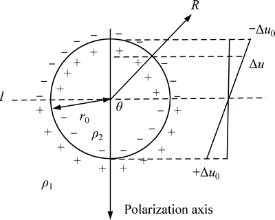
Fig. 1 A polarized sphere

           (1)

The potential of any point on line l is zero, the maximum ±ΔU₀ exists in the direction of the polarization axis, and the normal component of current density is continuous. Then the self-potential of any point in the space can be calculated as

                    (2)

If the polarization axis is rotated an angle α about the negative x axis, as shown in Fig. 2(a), then the self- potential at the ground surface can be given by

                (3)

In a similar way, the self-potential induced by a cylinder which extends to infinity can be obtained by solving the Laplace equation using a cylindrical coordinates system. Then the self-potential equation for a global anomaly can be written as

                 (4)

where K is the electric dipole moment, z is the depth of the anomaly, α is the polarization angle, x₀ is the origin of the anomaly, and q is the shape factor. The shape factors are 1.5, 1.0 and 0.5 for a sphere, horizontal cylinder and a semi-infinite vertical cylinder, respectively.

In Fig. 2(c), an inclined sheet extends to infinity in a homogeneous medium with resistivity ρ. The potential distribution induced by this sheet is equivalent to that induced by a current dipole. So, the corresponding self-potential at the ground surface can be given by

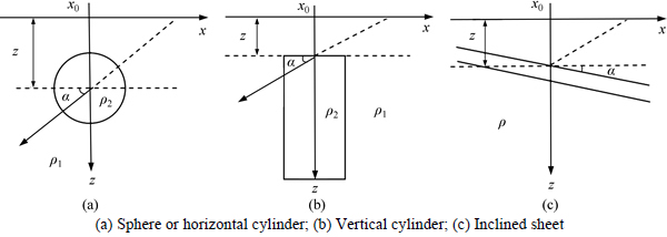
Fig. 2 Models of self-potential anomalies:

                            (5)

where r₁ and r₂ denote the distance from any point on the ground to both ends of the sheet, respectively, and I is the current of unit length. Using a coordinate transformation, Eq. (5) can be written as

     (6)

where α is the angle of inclination of the sheet and is also the polarization angle; α is the half length of the inclined sheet; x₀ is the origin of the center of the sheet; and z is the depth to the center of the sheet.

3 Intelligent optimization inversion algorithms

The goal of self-potential data inversion is to estimate the model parameters of a corresponding anomaly by minimizing the value of a given objective function. Four different naturally-inspired algorithms, GA, SA, PSO and ACO are adopted to design corresponding inversion algorithms and perform the estimations. For the convenience of comparison and evaluation, the same search-space and objective function, defined by Eq. (7), are used with all the intelligent optimization algorithms mentioned above:

                 (7)

where V_i denotes the measured self-potential data, and V(x_i) are the forward data.

For the same reason, all inversion results are evaluated by the same error formula as follows:

                    (8)

where M is the misfit.

3.1 Simulated annealing algorithm

The SA algorithm is a single state stochastic optimization, which is analogous to a cooling process controlling the crystallization of a melt in metallurgy. At each step, the SA heuristic considers some neighboring states of the current state, and probabilistically decides between moving the system to one of the neighboring states or staying in the current state. These probabilities ultimately lead the system to move to states of lower energy. Typically this step is repeated until the system reaches a state that is good enough for the application, or until a given computation budget has been exhausted. Finally, a good approximation to the global optimum of a given function in a large search space will be located.

The SA inversion algorithm for self-potential data is as follows:

1) Set a search-space, the initial temperature T, the maximum allowed number i of the same temperature, and the maximum number t_max of iterations.

2) Initialize a model m₀ in the candidate solution space.

3) Update the model parameters by the Metropolis sample rule:

Let ΔQ=Q(m)-Q(m₀). If ΔQ<0, the new model m will be accepted, otherwise the new model will be accepted according to the probability P=exp(-ΔQ/T), where Q(m) is the objective function. After a new model is accepted, let m₀=m and Q(m₀)=Q(m).

4) Under temperature T, repeat step 3) until the model is accepted i times.

5) Reduce the temperature T.

6) Repeat steps 3), 4) and 5), until the maximum number of iterations, t_max, is reached or a solution with adequate objective function value is found, then output the inversion results.

3.2 Genetic algorithm

The GA is a search heuristic that mimics the process of natural selection. It is routinely used to generate useful solutions for optimization and search problems. In a GA, a population of candidate solutions (individuals) to an optimization problem is evolved toward better solutions. Each candidate solution has a set of properties which can be mutated and altered. The evolution usually starts from a population of randomly generated individuals, and is an iterative process, with the population at each iteration called a generation. In each generation, the fitness of every individual in the population is evaluated; the fitness is usually the value of the objective function in the optimization problem being solved. More fit individuals are stochastically selected from the current population, and each individual’s genome is modified to form a new generation. The new generation of candidate solutions is then used in the next iteration of the algorithm. Commonly, the algorithm terminates when either a maximum number of generations has been produced, or a satisfactory fitness level has been reached for the population.

The GA inversion algorithm for self-potential data is as follows:

1) Set a search-space, the population size N, the crossover probability P_c, mutation probability, and the maximum number of iterations, t_max.

2) Initialize a population of individuals in the candidate solution space:m₁, m₂, …, m_N.

3) Calculate the fitness of every individual by equation F_it(x)=Q_max(x)-Q(x).

4) Produce a new population based on the GA operators: selection, crossover and mutation.

5) Repeat steps 3) and 4) until the maximum number of iterations, t_max, is reached or a solution with adequate objective function value is found, then output the inversion results.

3.3 Particle swarm optimization algorithm

The PSO is a population based optimization algorithm by mimicking the social behavior of individuals while searching for food as a member of the swarm. PSO optimizes a problem by having a population of candidate solutions, named particles, and moving these particles around in the search-space according to simple mathematical formulae over the particle’s position and velocity. Each particle’s movement is influenced by its local best known position, but it is also guided toward the best known positions in the search- space which are updated as better positions are found by other particles. This is expected to move the swarm toward the best solutions.

The PSO inversion algorithm for self-potential data is as follows:

1) Set a search-space, the populations size N, and the maximum number t_max of iteration.

2) Initialize a population of particles with location X and velocity V in the candidate solution space, and initialize the particle’s best known position p^t to its initial position.

3) Evaluate particles by objection function Q(m), get the swarm’s best known position g^t.

4) Update the particle’s velocity and location through

         (9)

                               (10)

where W^t is the inertia, and are velocity factors, p^t is the particle’s best known position, g^t is the swarm’s best known position, and R₁ and R₂ are vectors of random numbers uniformly distributed on (0, 1).

5) Update the particle’s best known position p^t+1 and the swarm’s best known position g^t+1 by evaluating particles using the objective function Q(m).

6) Repeat steps 4) and 5) until the maximum number of iterations, t_max, is reached or a solution with adequate objective function value is found, then output the inversion results.

3.4 Ant colony optimization algorithm

The idea of the ACO algorithm is to mimic the behavior of ants seeking a path between their colony and a source of food. The path of an ant can be considered as a candidate solution for an optimization problem. Ants lay down pheromones on trails while seeking paths. All ants are likely to follow the pheromone and reinforce it. Finally a path with the highest pheromone density, which will also be a global optimal solution to the corresponding optimization problem, will be obtained because it has been marched over more frequently than others.

The ACO inversion algorithm for self-potential data is as follows:

1) Set a search-space, the population size N, the maximum number (N_max) of searching, and the maximum number of iterations, t_max, of search-space.

2) Discretize the search-space and form a matrix of order n×(N_ep+1), where n is the number of parameters to be solved in the inversion, N_ep is the number of equal parts one parameter search-space being discretized into. Initialize a pheromone matrix τ_ij of order n×(N_ep+1) with the identity matrix I.

3) Form ant populations m₁, m₂, …, m_N based on probabilities given by Eq. (11) while discretizing the search-space:

                         (11)

where N_fss is the subdivision number of feasible solution space

4) Update the pheromone matrix τ_ij through Eqs. (12) and (13) as

        (12)

                       (13)

where Q is the objective function, and β is a constant.

5) Repeat steps 3) and 4) until the maximum number N_max is reached, output the current optimal model x^t according to the pheromone matrix.

6) Decrease the search-space and repeat steps 3), 4) and 5) until the maximum number of iterations, t_max, is reached, then output the inversion results.

4 Numerical experiments

Firstly, the synthetic data calculated from single self-potential anomaly model are employed to perform the inversion. The model I is a vertical cylinder with corresponding model parameters (z=5 m, q=0.5, θ=60°, K=500 mV, x₀=2 m).

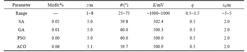
All the results searched by the 4 inversion algorithms are shown in Fig. 3 and Table 1. There is no obvious difference between the inversion results from different algorithms while inverting synthetic data from single anomaly model.

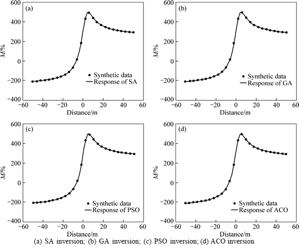
Fig. 3 Match between inversion results and synthetic data from model I:

Table 1 Inversion parameters of synthetic data from model I

Secondly, synthetic data calculated from a multi-anomaly model is tested using these inversion algorithms. Model II includes a sphere with corresponding model parameters (z=5 m, q=1.5, θ=30°, K=12000 mV, x₀=-50 m), and an inclined sheet with parameters (z=20 m, a=10 m, θ=40°, x₀=15 m, K=150 mV).

The inversion results of model II are shown in Fig. 4 and Table 2. There is also no obvious difference between the inversion results from the different algorithms while inverting synthetic data from the multi-anomaly model.

To evaluate the inversion performance, the mean relative errors of model parameters are determined and the computation times are recorded in the tests. As shown in Table 3, all the mean relative errors of the 4 algorithms are small. That means that all of these intelligent algorithms can provide reliable inversion results with sufficient accuracy. It is worth pointing out that the PSO algorithm has far smaller mean relative error than the other algorithms. The statistics of computation times also demonstrate the PSO algorithm’s competitive advantage in inverting self-potential data. The characteristic of less time consuming may result from the good convergence speed of PSO, as shown in Fig. 5.

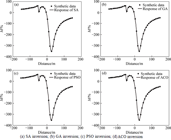
Fig. 4 Match between inversion results and synthetic data from model II:

Table 2 Inversion parameters of synthetic data from model II

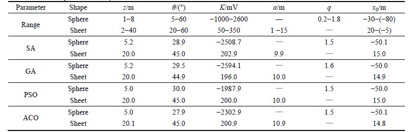
Table 3 Comparison of mean relative errors and inversion times

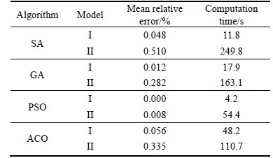
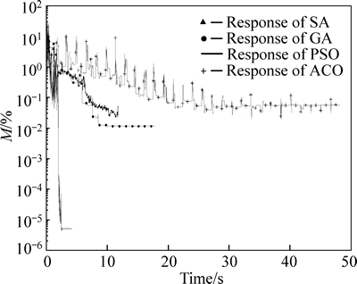
Fig. 5 Variation of relative error with time

For an intelligent optimization algorithm, it is very important to explore the candidate solution space with good balance between global and local searching. This capability means that the algorithm can not only search the space thoroughly but also provide good convergence speed guarantee. In the inversion of model I, the parameter K is selected deliberately to perform algorithm analysis for its large search-space. Figure 6 shows the distribution of inversion misfit of parameter K in the inversions for model I. As shown, the value of K appears everywhere in the whole space in all inversions. That means the algorithms all have good global searching ability. Comparing the distributions with the 3 other algorithms, the distribution of the PSO concentrates more upon the optimal value. It shows that the PSO has a better balance between global and local searching. This characteristic makes the PSO avoid too much irrelevant searching and find the optimum more quickly.

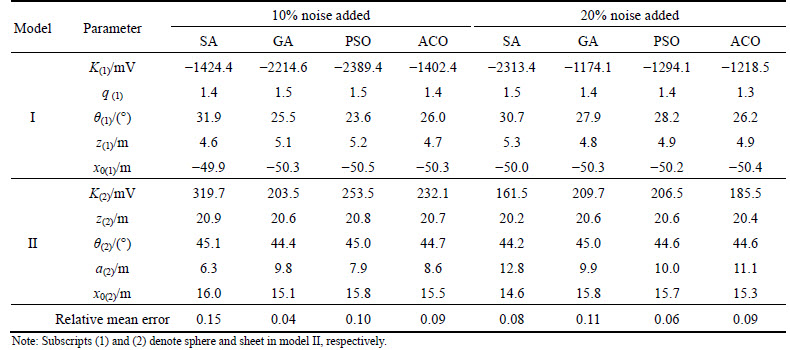
Lastly, noise added synthetic data are used to test these inversion algorithms. Good tolerance to noise is also an important capability for a robust inversion algorithm white gaussian noise (10% and 20% of the average value of the data, respectively) is added into the data forwarded from models I and II. Then these noise-added synthetic data are inverted by the 4 algorithms, respectively. As shown in Figs. 7 and 8, all inversion responses match the true model data very well. Table 4 shows the values of inverted parameters of model II in detail, which demonstrates the 4 inversion algorithms all have good tolerance to noise. At this point, there is no obvious difference between these algorithms.

5 Conclusions

Four intelligent optimization algorithms, SA, GA, PSO and ACO are employed, to invert the self-potential data, and assessed the performance of the algorithms. During the numerical tests with noise-free and noise- added synthetic data, the 4 algorithms all provide model parameters very close to the true ones. That indicates these intelligent algorithms have the capability to invert self-potential data reliably even when given a large search-space. The noise-added data tests also prove these inversion algorithms are robust and tolerant to noise. This is significant for inverting self-potential data, which is the one of the geophysical responses most easily affected by noise. Furthermore, the PSO algorithm is distinguished from the others for its higher precision of inversion and less computation time. The reason is that the PSO has better balance between global and local searching. It can search the whole solution space thoroughly and also have fast convergence at the same time. Among these four algorithms, the PSO is fastest. These advantages make PSO a powerful technique to invert self-potential data in cases where a priori information is insufficient or even not available.

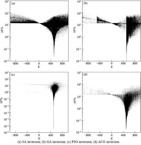
Fig. 6 Distribution of misfits of inverted value of K during iteration:

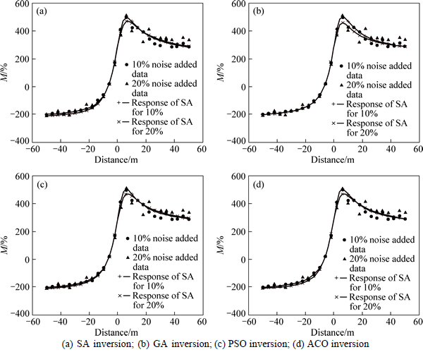
Fig. 7 Match between inversion results of noise added data and synthetic data from model I:

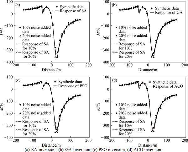
Fig. 8 Match between inversion results of noise added data and synthetic data from model II:

Table 4 Inversion parameters of noise added synthetic data from model II

Acknowledgments

We acknowledge Professor David Nobes for helping improve the English expression.

References

[1] de CARLO L, PERRI M T, CAPUTO M C, DEIANA R, VURRO M, CASSIANI G. Characterization of a dismissed landfill via electrical resistivity tomography and mise-à-la-masse method [J]. Journal of Applied Geophysics, 2013, 98(11): 1-10.

[2] JARDANI A, REVILl A, SANTOS F A M. Detection of preferential infiltration pathways in sinkholes using joint inversion of self-potential and EM-34 conductivity data [J]. Geophysical Prospecting, 2007, 55(5): 749-760.

[3] ABDELRAHMAN E M, ESSA K S, ABO-EZZ E R. New least-square algorithm for model parameters estimation using self- potential anomalies [J]. Computers & Geosciences, 2008, 34(11): 1569-1576.

[4] ABDELRAHMAN E M, EL-ARABY H M, EL-ARABY T M. New methods for shape and depth determinations from SP data [J]. Geophysics, 2003, 68(4): 1202-1210.

[5] FERNANDEZ-MARTINEZ J L, GARCIA-GONZALO E, FERNANDEZ-ALVAREZ J P, KUZMA H A, MENENDEZ-PEREZ C O. PSO: A powerful algorithm to solve geophysical inverse problems application to a 1D-DC resistivity case [J]. Journal of Applied Geophysics, 2010, 71(1): 13-25.

[6] WANG R, YIN C, WANG M, WANG G. Simulated annealing for controlled-source audio-frequency magnetotelluric data inversion [J]. Geophysics, 2012, 77(2): E127-E133.

[7] SHARMA S P, BISWAS A. Interpretation of self-potential anomaly over a 2D inclined structure using very fast simulated-annealing global optimization-An insight about ambiguity [J]. Geophysics, 2013, 78(3): WB3-WB15.

[8] BISWAS A, SHARMA S P. Optimization of self-potential interpretation of 2-D inclined sheet-type structures based on very fast simulated annealing and analysis of ambiguity [J]. Journal of Applied Geophysics, 2014, 105(2): 235-247.

[9] BALKAYA C. An implementation of differential evolution algorithm for inversion of geoelectrical data [J]. Journal of Applied Geophysics, 2013, 98(3): 160-175.

[10] SONG X, LI L, ZHANG X, HUANG J, SHI X, JIN S, BAI Y. Differential evolution algorithm for nonlinear inversion of high-frequency Rayleigh wave dispersion curves [J]. Journal of Applied Geophysics, 2014, 109(10): 47-61.

[11] BIJANI R, PONTE-NETO C F, CARLOS D U, SILVA-DIAS F J S. Three-dimensional gravity inversion using graph theory to delineate the skeleton of homogeneous sources [J]. Geophysics, 2015, 80(2): G53-G66.

[12] GRUTAS R, YAMANAKA H. Shallow shear-wave velocity profiles and site response characteristics from microtremor array measurements in Metro Manila, the Philippines [J]. Exploration Geophysics, 2012, 43(4): 255-266.

[13] FERNANDEZ-MARTINEZ J L, GARCIA-GONZALO E, NAUDET V. Particle swarm optimization applied to solving and appraising the streaming-potential inverse problem [J]. Geophysics, 2010, 75(4): WA3-WA15.

[14] FERNANDEZ-MARTINEZ J L, MUKERJI T, GARCIA- GONZALO E, SUMAN A. Reservoir characterization and inversion uncertainty via a family of particle swarm optimizers [J]. Geophysics, 2012, 77(1): M1-M16.

[15] ZHU Xiao-xiong, CUI Yi-an, LI Xi-yang, TONG Tie-gang, JI Tong-xin. Inversion of self-potential anomalies based on particle swarm optimization [J]. Journal of Central South University: Science and Technology, 2015, 46(2): 579-585. (in Chinese)

[16] PEKSEN E, YAS T, KAYMAN A Y, OZKAN C. Application of particle swarm optimization on self-potential data [J]. Journal of Applied Geophysics, 2011, 75(2): 305-318.

[17] SONG X, TANG L, LV X, FANG H, GU H. Application of particle swarm optimization to interpret Rayleigh wave dispersion curves [J]. Journal of Applied Geophysics, 2012, 84(9): 1-13.

[18] PALLERO J L G, FERNANDEZ-MARTINEZ J L, BONVALOT S, FUDYM O. Gravity inversion and uncertainty assessment of basement relief via particle swarm optimization [J]. Journal of Applied Geophysics, 2015, 116(3): 180-191.

[19] YAN Z, GU H, CAI C. Automatic fault tracking based on ant colony algorithms [J]. Computers and Geosciences, 2013, 51(02): 269-281.

[20] LIU S, HU X, LIU T, XI Y, CAI J, ZHANG H. Ant colony optimization inversion of surface and borehole-magnetic data under lithological constraints [J]. Journal of Applied Geophysics, 2015, 112(1): 115-128.

[21] EL-KALIOUBY H M, AL-GAMI M A. Inversion of Self-potential anomalies caused by 2D inclined sheets using neural networks [J]. Journal of Geophysics and Engineering, 2009, 6(1): 29-34.

(Edited by FANG Jing-hua)

Foundation item: Project(41574123) supported by the National Natural Science Foundation of China; Project(2015zzts250) supported by the Fundamental Research Funds for the Central Universities, China; Project(2013FY110800) supported by the National Basic Research Scientific Program of China

Received date: 2015-07-30; Accepted date: 2015-12-04

Corresponding author: CUI Yi-an, PhD, Associate Professor; Tel: +86-731-88877075; E-mail: cuiyian@csu.edu.cn