J. Cent. South Univ. (2018) 25: 2199-2218

DOI: https://doi.org/10.1007/s11771-018-3908-3

A method of searching fault propagation paths in mechatronic systems based on MPPS model

WANG Yan-hui(王艳辉)^{1, 2, 3}, LI Man(李曼)^{1, 2, 3}, SHI Hao(史浩)^{1, 2}

1. State Key Laboratory of Rail Traffic Control and Safety, Beijing Jiaotong University, Beijing 100044, China;

2. School of Traffic and Transportation, Beijing Jiaotong University, Beijing 100044, China;

3. Beijing Research Center of Urban Traffic Information Sensing and Service Technology,Beijing Jiaotong University, Beijing 100044, China

Central South University Press and Springer-Verlag GmbH Germany, part of Springer Nature 2018

Abstract: In view of the structure and action behavior of mechatronic systems, a method of searching fault propagation paths called maximum-probability path search (MPPS) is proposed, aiming to determine all possible failure propagation paths with their lengths if faults occur. First, the physical structure system, function behavior, and complex network theory are integrated to define a system structural-action network (SSAN). Second, based on the concept of SSAN, two properties of nodes and edges, i.e., the topological property and reliability property, are combined to define the failure propagation property. Third, the proposed MPPS model provides all fault propagation paths and possible failure rates of nodes on these paths. Finally, numerical experiments have been implemented to show the accuracy and advancement compared with the methods of Function Space Iteration (FSI) and the algorithm of Ant Colony Optimization (ACO).

Key words: mechatronic systems; complex networks; fault propagation path; maximum-probability path search (MPPS)

Cite this article as: WANG Yan-hui, LI Man, SHI Hao. A method of searching fault propagation paths in mechatronic systems [J]. Journal of Central South University, 2018, 25(9): 2199–2218. DOI: https://doi.org/10.1007/s11771- 018-3908-3.

1 Introduction

1.1 Background

Many technical processes and products in mechanical and electrical engineering are showing an increasing integration of mechanics with digital electronics and information processing, which is called the mechatronic system [1]. For example, spacecraft systems and high-speed trains are respectively assembled from thousands of components, with complex system structures and increasing integration leading to dependencies in function. These features are fundamental factors affecting fault propagation. Failure of one or more components could spread and extend on a large scale, with even a minor fault resulting in catastrophic consequences. The increasing complexity in the design of mechatronic systems challenges the applicability of rule-based designs and classical techniques of failure analysis. Therefore, understanding the fault propagation process can support fault diagnosis, which is essential for the process safety, efficient operation, and maintenance management of systems [1, 2].

1.2 Related literature

A fault is an abnormal state of a machine or a system, including a dysfunction or malfunction of a part, an assembly, or even the entire system.According to the scope of what is affected by a fault, it can be classified into local fault and propagation fault [3]. The former only causes a breakdown of the component itself, with no effect on other components. The latter not only makes the component abnormal but also affects others, which may result in more serious consequences. In a system, a fault is propagated among components by an action relationship, and it is related to the physical structure and the process of function implementation. The importance of fault propagation analysis to safeguard system safety has motivated much research toward the description of the failure propagation process. Over the past decades, the problem of failure propagation, which is included in the framework of cascading failure and path optimizations, has attracted tremendous attention from numerous researchers.

The complex network theory, with a summarization of the features concerning complex systems, has been employed as a mathematical description in many fields [4]. The application of the network theory, in which systems are represented by nodes and edges with varying characteristics and distributions, helps us to model and understand the nature of failure propagation. To predict the failure propagation in complex networks, two types of simulation models have been built, namely probabilistic models and complex network models [5].

1) The probabilistic models, which include fault tree analysis (FTA), failure mode and effects analysis (FMEA), and Bayesian networks (BNs), in a broad sense [6], do not depend on the topologic characteristics of networks. AMRANI et al [6] presented an overview of all the quantitative and qualitative methods and evaluated their significance for mechatronic system reliability studies. A hybrid FTA and FMEA were applied by SHARMA et al [7] to examine the risks and to study the reliability of a complex mechatronic system. CHOLEY et al [8] used the FMEA and FTA to identify and reduce risks with reference to system safety critical structures and behaviors. Relevant reliability parameters and indices using BN, which are converted by a dynamic fault tree, were calculated [9]. In Ref. [10], an improved Markov chain method, which was aimed at reducing the scale of a problem, was used to deal with the reliability of a mechatronic subsystem that controlled an unmanned aerial vehicle flight.

2) Complex network models adopt the graph theory to characterize the topological properties of components, which are used to describe the loads, and the entire network. A model had been proposed for vulnerability analysis of nodes to identify the relevant key nodes and preliminary vulnerabilities of systems, and to focus further on a detailed analysis of the failure propagation in the network [11–15]. WANG et al [16] proposed a cascading model based on a rule of load local redistribution to examine cascading failures in a typical network, i.e., the BA network with a scale-free property. YADAV et al [17] adopted the concepts of node degree and betweenness to the cascading failure analysis in small-world, scale-free, and local-world networks respectively. In reliability, the statistical properties of the topological structure of a system have been analyzed with a small-world network as well as a fault propagation model based on a small-world clustering proposed in Refs. [11, 18]. AHMAD et al [19] used the information matrices from a graph theoretic approach to obtain minimal cuts and calculated the system reliability using failure rates of nodes. In Ref. [20], Dijkstra’s algorithm was selected to predict the shortest path of a mechatronic system containing interrelated faults, effects, and causes. YAO et al [21] presented a novel graphical representation of a module signal diagram to construct a signal fault propagation tree and fault propagation tree of a four-rotor unmanned helicopter. Instead of using a probabilistic method, the fault propagation intensity with respect to the statistical information of the network was defined as the weight of the edge between nodes, and then the fault propagation paths with high risks were obtained [18]. The cause-and-effect relationships among components were mapped for the relationships among nodes in a complex network, and the search method of the failure propagation path from the source nodes to the target nodes was studied with the application of node coordinate connections of an electrical control system [13]. From the above studies, the theory of complex networks can be practical for application and simulation of complex system techniques in an effort to hamper the propagation of faults.

Methods such as FTA and FMEA have been commonly used for failure analysis [8, 22]. FTA is a top-down method, which is applied to map the relationship between events such as subsystem failures and their causes [22, 23]. However, FTA has typically been constructed by engineers under different scenarios [2, 19]. In FMEA, analysts drew up some lists of component failure modes to deduce the effects of those modes in the system [24]. However, the intelligent part of the FMEA process remains a manual and laborious process with a mere consideration of single point failures in a system in general [25, 26]. Both FTA and FMEA are very time-consuming for a thorough analysis with an application to the local system, rendering them unsuitable in many cases [6]. With the use of probabilistic intermediate nodes instead of gates, BN can model the dependencies between components in a more flexible manner to show more than two states of node values, which can make it an alternative [27–29]. Even though BNs are powerful, the construction of BN systems is cumbersome and more difficult than that of FTA. The major difficulties of fault propagation analysis involve identification of faults, causes, and consequences in a systematic manner. The above- mentioned models require information on failure modes and effects of components or systems, which are considerably expensive to acquire in general. With the advancement in structure and integration, system components are increasing, with each component interacting with others in a nonlinear way. Thus, it is necessary to find methods of exploring the behavior of systems. The emergence of complex network techniques and applications has necessitated the development of fault propagation models.

Although the above-mentioned studies involved fault propagation from multiple aspects, there are some problems:

1) The existing methods [8, 9, 27–29] are time-consuming and mainly focus on failure events, failure modes, and fail-out, which usually call for specialized knowledge and engineering experience, owing to ignorance of system microelements and the effect of action relationship among them.

2) The application of the complex network theory, with systems represented by linking nodes and edges with varying characteristics and distributions, helps us to model and understand the features of fault propagation. However, more attention on the analysis of fault propagation has been paid to the topological characteristics of nodes and edges [11, 12–16, 18, 30], with a consequent ignorance of the reliability features of components and links in networks.

3) Regarding the fault propagation path in a complex system, existing research mostly concentrates on a certain path [11, 18], and only few studies focus on an in-depth analysis of the competition and selection mechanism of other paths.

1.3 Contributions

In light of the above problems, this study investigates the mechanism of fault propagation and the propagation paths based on the properties of the failure of system elements and the topology of complex network. The contributions are summarized as follows:

1) In order to describe the structural and action behavior of the mechatronic system’s components, a system structural-action network (SSAN), which is simpler, is proposed, in an effort to study the fault propagation from the micro perspective of the system.

2) To synthetically consider the reliability and topology properties, the fault propagation properties of nodes and edges are proposed. The fault properties based on failure data are predominant in the propagation process, but a failure data sample is difficult to obtain. The topology properties are used to revise the fault properties. The new properties which consist of fault and topology can overcome the deficiency of data samples.

3) With the purpose of analyzing the multi- fault propagation path sequence, the maximum- probability path search (MPPS) method is proposed to determine all propagation paths based on the selection rules, with an illustration of constraints.

The rest of this paper is organized as follows. Section 2 introduces the SSAN model and presents the methods of calculating the propagation properties of nodes and edges. The mechanism of path propagation and selection in the network is analyzed as presented in Section 3. In Section 4, the MPPS method, which is designed to address the problem of path searching, is introduced. Numerical experiments are implemented, as described in Section 5, for demonstrating the efficiency and effectiveness of the proposed approach compared to the function space iteration (FSI) method and ant colony optimization (ACO). Conclusions are drawn as presented in the last section.

2 System structural-action network (SSAN)

This study focuses on how to determine all propagation paths after one or more component faults occur in a mechatronic system and investigates changes in possible failure rates of nodes on paths. The assumptions here are as follows:

1) In mechatronic systems, components can be classified into two categories. One is the mechanical component and the other is the electronic one. Therefore, the life distribution of components agrees with the Weibull and exponential distributions respectively.

2) As the propagation time is determined by distance, it is difficult to determine the speed and medium at present. Here, the propagation time on the edges is ignored and the distance of each edge is assumed as 1 in this study.

3) A node is completely failed when the failure path is derived, and all components are considered as nonrepairable.

To construct a mathematical model for the problem, the applicable symbols are listed in Table 1 and the others are given in the text.

2.1 SSAN model

Mechatronic systems are composed of modular units, which consist of items with each item having smaller components. For example, in Figure 1, a car is a complex mechatronic system, and the engine can be regarded as a unit. The engine consists of items such as the piston assembly and carburetor. A piston assembly as an item is composed of components such as the piston, pin, and crankshaft [31]. The core of the engine control unit is a general-purpose microprocessor or a large-scale integrated circuit specifically designed for automotive engines. A component is a physical structure, which is composed of individual parts. Major failures originate from a component and then spread to other components via propagation paths. Hence, a component must be regarded as the basic element of a network.

Another key element in the network is the edge between nodes. For example, in the system structure, if the weld that fixes the components together is corrupted, an accident could occur. A connection is a part of the physical structure of a system that transmits the action relationship to fulfill a specific function. In other words, a physical connection serves as the carrier of the action relationship. For example, the braking process is completed through the pedal and retarding disk when the vehicle brakes and the force is transmitted via the connection. In this study, this connection is defined as the edge in the network.

Table 1 Meaning of symbols used

A complex network is a set of nodes with connections among them, and similarly, a system is composed of components and connections. When a system is represented by a network, it is called SSAN. SSAN is modeled as a graph, G=(V, E) as Figure 2 shows, where V is a finite set of nodes and E is a finite set of directed edges between the corresponding nodes. e_ij means that the action relationship is triggered from v_i to v_j and e_ji is opposite to e_ij. The edge between nodes depends on the physical structure, whereas the directivity relies on the action relationship. An unidirectional edge means that the action relationship is unidirectional and a bidirectional one means that the action relationship is mutual.

Figure 1 System structure of a car

Figure 2 SSAN graph

2.2 Properties of fault propagation in network nodes

The properties of topology and failure are investigated to obtain a fusion characterization of nodes. In the following sections, the recommended properties are shown.

1) Topologic property of node

Numerous studies have revealed that almost all real networks, such as social networks, world wide web, electrical power grids, and electromechanical systems, present a small-world effect [18–20], which has an obvious implication for the propagation of processes taking place in the networks. For instance, if one considers the spread of message, energy, or actually anything else across a network, a small-world effect implies that the spread will be rapid. The topological structure and network environment determine some important factors of fault propagation according to Refs. [11, 13, 18]. A well-known property is that, on average, pairs of nodes can be connected by short path lengths [4]. Another property is the clustering coefficient, which means a higher likelihood of any two nodes with a common neighbor connected [32]. The clustering coefficient affects the extent (or scope) of fault propagation and the characteristic path length to depth [18]. In fact, the clustering of node i depends on the degree, particularly the out- degree in a directed network. Figure 3 illustrates the degree of in-degree and out-degree of v_i. The degree of node v_i is defined as the total number of edges connecting v_i, whereas the out-degree (d_i) is the number of edges originating from v_i. For example, in Figure 3, the degree of node v_i is n and the out-degree is (n-m). A larger out-degree of a node corresponds to more propagation routes, with a greater spread scope, just as one might expect intuitively [18].

Figure 3 Illustration of degree and out-degree of v_i

Node betweenness has been studied in the past as a measure of centrality and influence of nodes in networks. In Ref. [33], the load, i.e., the topologic property of a node, was defined as the total number of shortest paths passing through the node betweenness. However, the calculation of betweenness requires a global information of the network and takes o(n²) time [34], which is resource-consuming compared to the out-degree. In order to reduce computation, the out-degree of a node can be regarded as a topologic property. Because the value of out-degree is 0 or other positive integer, the topologic property s_i is normalized as in the following:

                              (1)

where n is the total number of nodes in the network and 0≤s_i≤1.

2) Property of node failure

A failure rate is an intuitive index to reflect the function integrity of a component, and therefore, the failure property of a node places an emphasis on it.

The failure rate is the frequency at which an engineered system or component fails, and is expressed, e.g., in failures per hour. The failure rate of a component typically depends on time, with the rate varying over the life cycle of the component. For example, a crankshaft’s failure rate in its fifth year of service may be many times greater than that during its first year of service, even if it has a higher cost of maintenance.

The failure behavior of a population of components (such as electronic and mechanical components) over their life cycle (i.e., from production to disposal) is commonly represented by the bathtub curve as shown in Figure 4. This figure shows how the overall failure rates of a component change with time. With the increase in life expectancy, the greater failure rate, the higher the chances of spreading.

Figure 4 Failure rate curve changing with time

3) Propagation property of node failure

If the topological and failure properties of nodes are obtained, the propagation property of v_i is defined as

                                (2)

where exp is a mathematical constant, i.e., e= 2.71828 and 1≤e^s_i≤ e. e^s_i is the coefficient that explains the amplification effect of the topological property of nodes on the propagation process of failure.

2.3 Properties of fault propagation in network edges

1) Topologic property of edge

In networks, each node contributes to the failure propagation in a way that cannot be replaced by the others. However, the edge is also critical because propagation paths are composed of edges. For a given network, at each step, fault, in the form of information, energy, etc., is exchanged between every pair of nodes and is subsequently transmitted along the shortest path connecting them [33]. The edge betweenness b_ij is often chosen as the definition of the topologic property of edge because betweenness directly measures the load of transmitting quantity in the process. The larger the load value of edge, the easier the occurrence of failure of nodes via this edge. Analogous to the node betweenness, the edge betweenness is defined as the number of shortest paths passing through it [18, 34]. To limit the value between 0 and 1, the edge topologic property S_ij of e_ij is normalized as follows:

                            (3)

where is the sum betweenness of all edges.

2) Property of edge failure

The property of edge failure represents the action relationship based on the feature of causality, which may trigger failure between adjacent components. Causality is a physical phenomenon based on a cause–effect relationship between different components. When one focuses on the interconnections of the components, the first step is to recognize the causality between them and that is what an engineer is interested in because one should find the fault selection paths. The cause– effect relationship means fault information transference [35], but it is not always available. Thus, another resource of analysis is historical data, which can effectively complement and facilitate the probabilistic property. However, the collection of sufficient data is still a challenge, making it necessary to take the topological property into consideration. To solve the problem, we need to acquire the data from both the manufacturer and the operator.

The edge failure property P_ij is defined as

                               (4)

whereis the fault frequency of v_j caused by the failure of v_i. Typically,and P_ij=P_ji, (0≤P_ij≤1).

3) Propagation property of edges

Nodes that fail in the system network will gradually spread to other ones. In the propagation process, failures will diffuse through edges that have a larger probability of propagation [5, 16]. However, it is difficult to obtain accurate information of probability in practice, particularly for a system that has a highly complicated structure and logical relationship. To solve the problem, the propagation property of edges instead of the failure property is defined and assigned to the edge as the coefficient [18]. The propagation property w_ij of e_ij is defined as

                            (5)

3 Paths of fault propagation in SSAN network

3.1 Path description of fault propagation

Here, the path problem of fault propagation is discussed. A walk, l={v_i, v_m, …, v_n, v_j}, in a network is a collection of sequential nodes, with each node being adjacent to the next node [17]. Therefore, the path of fault propagation is defined as a walk that does not repeat nodes. The first node along the path is called the initial fault node, and the last one in the path is called the destination node. There may be multiple paths from v_i to v_j and each path is defined as set l_ij={e_im, e_m1, …, e_nj}. The length p(l_ij) of the propagation path l_ij is defined as

               (6)

The most effective path (MEP) between two nodes is the one with the maximum length. To describe the possible failure rate of v_j, the rate R(j) is defined as

                          (7)

If v_i is not the initial fault point and v_d is an adjacent node of v_i, the length of the phased path l_id in the kth step is defined as

                      (8)

For example, Figure 5 illustrates a simple SSAN network with four nodes, with the indication of the propagation paths between v_i and v_j. l_ij={e_i1, e_1j} and l_ij={e_i2, e_2j} are the paths from the initial fault point v_i to the destination v_j.

Figure 5 Network with all propagation paths

3.2 Process of path selection

Faults spread along the edges and the influenced adjacent nodes are called the involved ones. The involved nodes are put with the same step to research in this study. Figure 6 shows the involved set of nodes F(~)_k+1={v₁, v₂, …, v_m}. If v_i is the initial failure point in the kth step, node set {v₁, v₂, …, v_m} and triggered paths set L(~)_k={l_i1, l_i2, …,l_im} belong to the (k+1)th step. If the MEP is l_i1, the possible failure node set is F_k+1={v₁}.

Figure 6 Illustration of distinction between kth step and (k+1)th step

The longer the path, the weaker the spread ability. In addition, the bidirectional edge between node pairs may result in the propagation into a cycle in some edges. Such type of search problems that affects the distance of traversing a path should be considered. According to Refs. [18, 36], the propagation process of faults is subject to the following constraints.

Hypothesis 1 The intensity of fault propagation will decrease by one order of magnitude when the number of propagation steps increases. The work by HAMMER [36] demonstrated that the node is safe when the intensity is less than 10^–8, which means that, along with the increase in the propagation steps, the fault propagation will be difficult to continue. Consequently, the failure will stop spreading in the kth step when the product of edge property attribute is less than 10^–8, that is

()                (9)

Hypothesis 2 If Eq.(9) is not met while all nodes have been traversed, the failure stops spreading.

Figure 2 shows an example for illustrating the above selection process. Suppose v_n and v₄ failed in the kth step, and then F_k={v₄, v_n}. Explicitly, in the (k+1)th step, the involved node set is{v₂, v₃}.

1) For v₂, the possible path is l_n2={e_n2}, and the MEP is l_k+1(v₂)=l_n2. Therefore, the length of the path from the possible failure node v_n in the kth step to the involved v₂ in the (k+1)th step is p(l_k+1(v₂))= p_k+1(lphase n2)=R(n)×w_n2.

2) With respect to v₃, the possible paths are l_n3={e_n3} and l₄₃={e₄₃}. To select the MEP l_k+1(v₃), we need to calculate the maximum length of all possible paths, i.e., p(l_k+1(v₃))p_k+1(lphase 43)}. In the case of p_k+1(lphase 43)>p_k+1(lphase n3), the MEP is l_k+1(v₃)=l₄₃; otherwise, l_k+1(v₃)=l_n3.

4 Search method of maximum- probability path

In this study, a novel approach to search the fault propagation paths in a network, i.e., the MPPS method, is proposed.

4.1 Operators of MPPS

In this subsection, three operators, which make the failure information conform to the propagation characteristics of the network, are required to model the MPPS method.

1) “” operator

Matrix A∈R^n×n and B∈R^1×n,

            (10)

2) “” operator

Matrix A∈R^n×n, B∈R^1×n, and B=(B^T)^T, where T is the transpose of a matrix,

           (11)

3) “” operator

Matrix A∈R^n×n and B∈R^1×n,

               (12)

where “” means the maximum.

4.2 Model of maximum-probability path search

The maximum-probability path (MPP) is one with the maximum length of all propagation paths. Aimed at searching for the MPP between the initial failure nodes and the destination ones, an obvious method is to find out all possible paths, with a subsequent selection of the best one from them. However, the spot of the search tree is considerably large in most cases and consequently it is extremely rigorous and cumbersome to find all possible paths. An intelligent method is useful in dealing with this problem. In many cases, the existing search technique can be improved with the use of guesses about the remaining lengths as well as facts about lengths already accumulated. Finally, if the guess about the remaining length is reliable, the length added to the already traversed one should be a good estimation of the total path length, i.e., d (total path length)=d′(already traveled)×d″(length remaining), where d′ (already traveled) is the known length, and d″ (length remaining) is the estimation of the remaining length. However, guesses are not perfect, and either overestimation or underestimation may cause the right path to deviate. In the MPPS path method, a prior guess of the remaining length is not necessary and the selection will be rectified in the iteration process.

The process of path selection results from information competition. In this method, the MPP lengths of paths and nodes with possible failure rates are obtained in each step.

The MPPS model consists of 8 elements.

            (13)

where f_k=[f_i]_1×n is the row matrix of node statuses and its value is either 0 or 1. When f_i=1, it means that v_i has become the failure position in the kth step; otherwise, v_i is normal.

In the (k+1)th step, the elements in the model are calculated as follows:

                           (14)

              (15)

where W_k is the transition matrix, which provides a selection for the path propagation from the kth step to the (k+1)th step.

To explain the meaning of Eq. (15), let

                         (16)

and

                         (17)

where Rnodes k+1 is the node possible failure rate in the kth step. Let matrix We k+1=[we ij], where i is the most probable node of fault in the kth step and j is a node, which is involved in the (k+1)th step, i.e., i∈F_k and we ij is the triggered probability of path l_ij. Here,and p(l_ij) can be acquired from The possible failure rates of nodes that belong to the set of G_k+1 are calculated according to Rnodes k+1 when the failure information is spread by paths infrom steps k to (k+1). Finally, the MEPs and the most possible failure rates of nodes are obtained with L_k+1 and F_k+1 taken into consideration.

The iteration process of the MPPS model mainly depends on the matrices and the predefined operations. Therefore, the model can be implemented through MATLAB. The block diagram of the logical structure is shown in Figure 7.

Figure 7 MPPS model framework

5 Numerical experiments and results

In this study, paths of fault propagation in networks and element properties are investigated with the use of two examples. One is a simple network, which is designed in Ref. [37] and the other is a network of a high-speed train system “CRHX.” The following sections describe the accuracy and superiority of the method compared to the FSI method and ACO algorithm respectively. Here, the MPPS model and FSI are used as shown in Figure 8.

Figure 8 SSAN network example

5.1 Accuracy verification

5.1.1 FSI method

The FSI method is used to search optimal paths in a directed network by defining a simple function, which is related to edge weights [36, 37]. The most possible route, whose value is the minimum, can be determined from all reachable paths when the weights of edges are known; however, the node properties are not considered in Ref. [37]. Thus, a simple function is developed properly to solve this problem, i.e., the definition of the edge property I_id in the FSI, which is

                              (18)

φm k(·) is defined as a simple objective function, where k is the number of iterations and m is the destination node. Let wFSI id be the weight of e_id and is defined as follows:

                     (19)

The length p^FSI(i, j) is the path length from v_i to v_j in the FSI method and it is defined as

                      (20)

The possible rate R^FSI(j) of v_j under different nodes as initial failure points is defined as

                      (21)

The FSI procedure can be performed in the following steps:

Step 1: Set the initial simple function, i.e., the length of a path.

        (22)

Step 2: Iteration. To determine the minimum path, the iteration function should be given. For each v (i=1, 2, …, n, i≠m), find

                (23)

Step 3: Repeat Step 2 until φm k+1(i)= where φm k+1(i) is the minimum path from v_i to v_m.

Step 4: Calculate the possible rate of R^FSI(m) of v_m.

5.1.2 Discussion of outcome

1) MPPS method

To demonstrate the MPPS method, assume that v₃ is the initial failure position in this example and determine the propagation paths from v₃ to another. Suppose that the failure rates of nodes are h=[h₁ h₂ h₃ h₄ h₅ h₆]=[1/8 1/7 1/6 1/2 1/4 1/3] respectively, with the topologic properties of nodes of s=[s₁ s₂ s₃ s₄ s₅ s₆]=[0.0667 0.2 0.2 0.2667 0.2 0.0667]. The topologic properties of edges are presented in Table 2.

Table 2 Topologic properties of edges

By using Eqs. (2) and (5), the propagation properties of nodes and edges are obtained as follows. The failure properties of nodes are U=[0.1336 0.1745 0.2036 0.6528 0.3054 0.3563]. Figure 9 shows three types of properties of nodes. The figure shows that v₄ has a high failure rate and out-degree, and with the use of the propagation property, the status of v₄ is raised, i.e., this node is crucial. Even though v₆ has a low out-degree, it has a high failure frequency to accelerate the fault of adjacent components, and a detailed description of the property of node is given with the use of this method.

Figure 9 Three types of node properties

The matrix W of edge propagation properties can be obtained by Eq.(5):

The procedure of the MPPS method can be executed as follows:

Step 1: From the assumption, we know that F₀={v₃}, f₀=[0 0 1 0 0 0], and M₀=[0 0 0.1833 0 0 0]. The initial transition matrix is obtained by Eq.(14):

Step 2: Let k=1, and calculateby Eq. (16):

Fromwe can obtain the involved node set of {v₁, v₄, v₅}, the possible path set of{l₃₁, l₃₄, l₃₅}, and the length of possible paths of p(l₃₁)= 0.0291, p(l₃₄)=0.0489, and p(l₃₅)=0.0245, respectively.

Step 3: Calculate Rnodes 1 using Eq. (17), with the possible failure rates of nodes obtained from Rnodes 1, i.e., R(1)=0.0028, R(4)=0.0188, and R(5)= 0.0063.

Step 4: Calculate M₁:M₁=[0.0028 0 0.1833 0.0188 0.0062 0]. It is known that the most possible failure node is F₁={v₁, v₄, v₅}; therefore, the most possible paths in the case of k=1 are L₁={l₃₁, l₃₄, l₃₅} and p₁(l₃₁)=0.02919, p₁(l₃₄)=0.0489, and p₁(l₃₅)=0.0245. The most possible failure rates are R₁(1)=0.0028, R₁(4)=0.0188, and R₁(5)=0.0063.

Step 5: Constraints checking. Obviously, there are nodes that have not been traversed. Check Hypothesis 1: ∏w_3j=0.2670×0.1172×0.1509> 10^–8 (j∈F₁). Consequently, the failure continues to spread.

Step 6: Let k=2 and repeat the above steps until one or both hypotheses are satisfied.

Figure 10 shows the results obtained with the MPPS method with v₃ as the initial failure point. All possible paths and MEPs with their lengths in each step are pointed out in Figures 10(a) and (b) respectively. In Figure 10(a), besides the MEP, there are other paths from k=1 to k=2. However, paths l₄₂ and l₄₆ are more satisfactory because their lengths are larger than the others. The most possible failure rates of nodes are obtained through the MEPs, i.e., R₂(2)=4.3044×10^–4 and R₂(6)=0.0011. Note that all nodes have been traversed in this case, and thus, the failure stops spreading. From the results, all propagation paths with their lengths and the possible failure rates of nodes are obtained.

The MEPs from different nodes, which serve as the initial failure point to v₅, are shown in Figure 10 (paths from v₃ to v₅) and Figure 11. The red lines in the figures are the MEPs, and the length of each path is also indicated in the figure.

All possible failure rates of nodes when different nodes act as the initial failure points are summarized in Table 3. The possible failure rates of nodes are derived when the MEPs are found.Figure 11 shows the corresponding paths to each node in the row. Note that the results of the MPPS method and FSI are practically equal, and their time complexities are both o(n²), where n is the total number of nodes.

2) FSI method

Table 4 presents the results of all MEPs and their lengths from v₁, v₂, v₃, v₄ and v₆ to v₅ with the FSI method. “a” and “v_j” of “a/v_j” in respectively represent the minimum path length and the node on the path from v_i to v₅. For example, 18118.6442/v₂ represents the length of the most possible path among all paths from v₁ to v₅, and v₂ is the node on the path. W ^FSI is the edge weight result with the FSI method. The minimum path lengths based on the FSI method are presented in Table 4.

Figure 10 Paths of failure propagation and their lengths with v₃ as initial failure point:

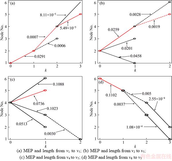
Figure 11 MEPs of different nodes, which are initial failure points:

Note that the results of the MPPS and FSI method are practically equal and their time complexities are both o(n²), where n is the total number of nodes. A comparison of the MPPS and FSI method is shown in Figure 12, where the x-axis is the initial failure point and the y-axis is the MEP length and the corresponding failure rates of v₅, respectively. The relative absolute errors of the path lengths are less than 0.6% and the failure rates of v₅ are less than 0.9%. As in the previous example, the results derived from the MPPS method seem to be an excellent approximation to the FSI results. In this case, the errors are mainly due to the operation. Interestingly, unlike in the FSI method, Figures 10 and 11 show that all paths and their lengths are obtained with other nodes as the initial failure points. Moreover, the MPPS exhibits some different features compared to the FSI method. It can be observed from Figures 10 and 11 that, along with the increase in k, several nodes become the “initial points,” i.e., the fault propagation results of multiple fault sources can be acquired in MPPS but no such phenomenon is observed in the FSI, which implies that the search method is helpful in solving the problem of failure propagation with multiple sources. In addition, the changes in failure rates of intermediate nodes on the MEPs can be observed from Table 3, implying that the MPPS method contributes to the investigation of the interaction among nodes. The nodes with high failure rates should get more protection or prevention. Compared to the FSI method, the MPPS is proven to be more exact and effective.

Table 3 Possible failure rates of nodes with different nodes as initial failure points

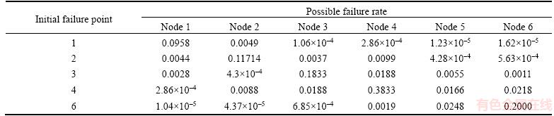
Table 4 Minimum path lengths based on FSI method

Figure 12 MEP lengths and comparison of most likely failure rates of node 5:

5.2 Advanced validation

A high-speed train is the typical mechatronic system, which is an integration of mechanics, electronics, computing, and automatic control [38], with more than 20000 components. Here, the power bogie subsystem is used to show the validity of the method and data are obtained from the actual operation fault collection of “CRHX” in China.

As Figure 13 shows, an SSAN network of the power bogie system with 35 nodes and 59 edges is established [39–41]. The names of the components are given in Table 5. The components and connections are represented by nodes and directed edges respectively.

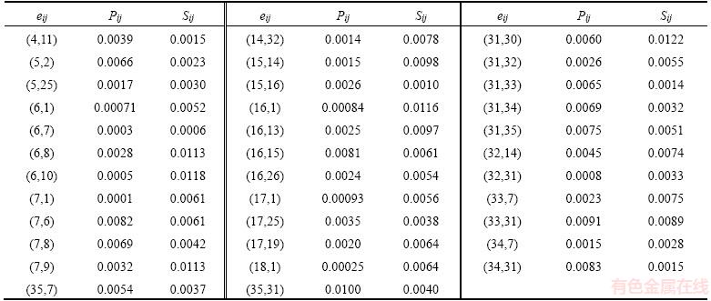
The data in Tables 6 and 7 are the topology and fault properties of the nodes and edges respectively. In Table 7, for example, (1,2) means e₁₂. In this example, a comparison is made between the ACO method and the MPPS.

Figure 13 SSAN network of power bogie system

Table 5 Names of components of power bogie system

Table 6 Node properties of power bogie system

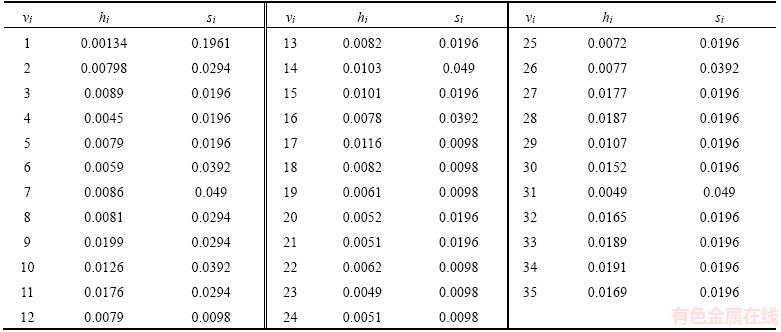
Table 7 Edge properties of power bogie system

Continued

5.2.1 Ant colony optimization

ACO is widely used because of its adaptable and robust performance in optimization problems. Moreover, it shows a good performance in avoiding local optima based on a higher diversification of the search [42, 43]. ACO is selected to carry out the research into the problem of failure propagation owing to its advantages. The target of ACO in this study is to find the propagation path that contains the highest length from the initial failure node to the presupposed destination. Thus, the objective function is given by

                  (24)

The objective function of the path optimization involves the maximum length, which is the product of elements; therefore, it is relatively difficult to solve the ACO algorithm. Hence, the objective function is replaced by the formula

               (25)

where “ln” is the natural logarithm symbol.

Furthermore, the objective function must be subjected to the following constraints [36]:

            (26)

where F_k is the set of nodes that are possibly affected by the kth step propagation.

Ants are sent out sequentially (not in parallel). Each ant iteratively starts from a node and adds new ones until all nodes have been visited. When in the kth step, an ant in node v_i applies the transition rule, i.e., it probabilistically selects the next node v_j from the set G_k+1.

The ant in node v_i chooses the next node v_j based on two factors: the heuristic information η_ij (here defined as I_ij; see section 5.1) and the pheromone trail τ_ij on the edge e_ij.

The next node v_j is chosen with a probability given by

             (27)

Because too much residual pheromone covers the heuristic residual information, the pheromone is updated when each ant has completed the entire travel of all nodes (which is the end of one cycle):

                     (28)

where ρ∈[0,1] is the evaporation rate and △τ_ij represents the increment of the pheromone in the cycle. Na is the total number of ants, whereas △τm ij is the quantity of the pheromone laid on the edge e_ij by the mth ant, and it is given as [3]:

     (29)

where Q is a constant and I_m means the value of the objective function of the mth ant.

5.2.2 Discussion of results

1) MPPS method

Suppose v₁₁ is the initial failure point. Then, the changes in the propagation paths and their lengths are investigated. Figure 14 shows all the possible paths as well as their lengths.

Figure 14 All possible paths when v₁₁ is initial failure point

Table 8 provides the possible failure rates of nodes in each step when v₁₁ is the initial failure point. Note that the failure propagation stops in the 4th step and there are no residual nodes that have not been traversed. At the same time, the product of path weights satisfies Hypothesis 1. From Figure 14, we know that the maximum length is 9.2×10^–19 and the MEP is v₁₁→v₁₄→v₁→v₂₅→v₅.

2) ACO algorithm

The objective function of the ACO algorithm is defined to maximize the length. It is necessary to identify all possible propagation paths from the initial failure point. The parameters applied in the ACO procedure are listed in Table 9. The best result obtained in the example is v₁₁→v₁₄→v₁→v₂₅→v₅ and the value of the objective function by Eq. (25) is -41.52.

The printed optimization process of the path search is shown in Figure 15, which reflects the change in the optimal value along with the iterations. The length of the path is e^–41.52= 9.2917×10^–19 and the possible failure rate of v₂₆ is h₅×e^–41.729=7.3404×10^–21.

Note that the MEP of the ACO is the same as that of the MPPS method. The relative absolute errors of the path length and the failure rate of node v₂₆ are less 0.9% and 1.2% respectively, which again suggests that the optimal searching path derived from the MPPS method seems to be fairly accurate. Although the results are practically equal, the ACO ignores the other paths and failure rates of nodes, which is a weak point.Furthermore, compared to the time complexity of ACO, which is o(n⁴), the MPPS method shows a higher efficiency and parallelizability.

Table 8 Possible failure rates of nodes

Table 9 Parameters of ACO algorithm

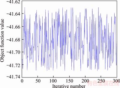
Figure 15 Optimization process of ACO

6 Conclusions

Fault propagation is a common phenomenon in real mechatronic systems owing to the uncertain selection and close connection between components. This study has proposed an efficient parallel model to determine the propagation path based on a system of directed network construction when component failure occurs. First, the proposed method allows a strong compatibility and serviceability in the use of the system and comparative analysis between different elementary components. It also provides a basic identification of weak components and links with specific and detailed analysis carried out in case of failure. Second, combining the topology properties and failure properties can accurately illustrate the dynamic and transfer feature of the failure information of the system. In the process of propagation, the properties of node and edge failures are more important than the topology attributes, which are used as correction factors, and highlight the influence of propagation in the network. In addition, the proposed method overcomes deficiencies of the conventional path selection.

The mathematical MPPS model is transformed with steps based on defined operators and all possible paths and their lengths are determined from the initial failure nodes to the others with this model. In future works, the partial failure of components, influence of propagation time, and more appropriate mechanism of competition for the failure should be studied.

References

[1] Isermann R. Mechatronic systems-innovative products with embedded control [J]. Control Engineering Practice, 2008, 16(1): 14–29. DOI: 10.1016/j.conengprac.2007. 03.010.

[2] Gabbar H A. Improved qualitative fault propagation analysis [J]. Journal of Loss Prevention in the Process Industries, 2007, 20(3): 260–270. DOI: 10.1016/j.jlp.2007. 04.010.

[3] WANG Chao-nan, XING Liu-dong, PENG Rui, PAN Zhu-sheng. Competing failure analysis in phased-mission systems with multiple functional dependence groups [J]. Reliability Engineering & System Safety, 2017, 164: 24–33. DOI: 10.1016/j.ress.2017.02.006.

[4] Newman M E J. The structure and function of complex networks [J]. SIAM Review, 2003, 45(2): 167–256.

[5] LI Yan-fu, Sansavini G, Zio E. Non-dominated sorting binary differential evolution for the multi-objective optimization of cascading failures protection in complex networks [J]. Reliability Engineering & System Safety, 2013, 111: 195–205. DOI: 10.1016/j.ress.2012.11.002.

[6] Amrani N B, Saintis L, Sarsri D, BARREAU M. Evaluating the predicted reliability of mechatronic systems: State of the art [J]. Mechanical Engineering: An International Journal, 2016, 3(2): 1–13.

[7] Sharma R K, Sharma P. Qualitative and quantitative approaches to analyse reliability of a mechatronic system: A case [J]. Journal of Industrial Engineering International, 2015, 11(2): 253–268.

[8] Choley J Y, Mhenni F, Nguyen N, BAKLOUTI A. Topology-based safety analysis for safety critical CPS[J]. Procedia Computer Science, 2016, 95: 32–39. DOI: 10.1016/j.procs.2016.09.290.

[9] Mi Jin-hua, LI Yan-feng, Yang Yuan-jian, PENG Wei-wen, HUANG Hong-zhong. Reliability assessment of complex electromechanical systems under epistemic uncertainty [J]. Reliability Engineering & System Safety, 2016, 152: 1–15. DOI: 10.1016/j.ress.2016.02.003.

[10] Martin C, Gonzalez-Prida V, Pérès F. Reliability assessment of a multi-redundant repairable mechatronic system [M]//Numerical Methods for Reliability and Safety Assessment. Springer International Publishing, 2015: 407–423.

[11] LIU Xiao-feng, AN Si-qi. Failure propagation analysis of aircraft engine systems based on complex network [J]. Procedia Engineering, 2014, 80: 506–521. DOI: 10.1016/ j.proeng.2014.09.108.

[12] FANG Xin-li, YANG Qiang, YAN Wen-jun. Modeling and analysis of cascading failure in directed complex networks [J]. Safety Science, 2014, 65(3): 1–9. DOI: 10.1016/ j.ssci.2013.12.015.

[13] YUAN Hai-bin. Network topology for the application research of electrical control system fault propagation [J]. Procedia Engineering, 2011, 15: 1748–1752. DOI: 10.1016/j.proeng.2011.08.326.

[14] Rocco C M, Ramirez-Marquez J E. Vulnerability metrics and analysis for communities in complex networks [J]. Reliability Engineering & System Safety, 2011, 96(10): 1360–1366. DOI: 10.1016/j.ress.2011.03.001.

[15] Johansson J, Hassel H. An approach for modelling interdependent infrastructures in the context of vulnerability analysis [J]. Reliability Engineering & System Safety, 2010, 95(12): 1335–1344. DOI: 10.1016/j.ress.2010.06.010.

[16] WANG Jian-wei, RONG Li-li, ZHANG Liang, ZHANG Zhong-zhi. Attack vulnerability of scale-free networks due to cascading failures [J]. Physica A: Statistical Mechanics and its Applications, 2008, 387(26): 6671–6678. DOI: 10.1016/ j.physa.2008.08.037.

[17] YADAV K, BISWAS R. An intelligent search path [J]. International Journal of Intelligent Systems, 2010, 25(9): 970–980. DOI: 10.1002/int.20434.

[18] GAO Jian-min, LI Guo, GAO Zhi-yong. Fault propagation analysis for complex system based on small-world network model [C]// Reliability and Maintainability Symposium (RAMS 2008). Las Vegas, USA: RAMS, 2008: 359–364. DOI: 10.1109/RAMS.2008.4925822.

[19] Ahmad A, Rizvi M A K, Al-Lawati A, MOHAMMED I, MALIK A S. Development of a MATLAB tool based on graph theory for evaluating reliability of complex mechatronic systems [C]// GCC Conference and Exhibition (GCCCE 2015). Muscat, Oman: GCCCE, 2015: 1–6. DOI: 10.1109/IEEEGCC.2015. 7060067.

[20] Hetmaczyk M P, wider J. The modified graph search algorithm based on the knowledge dedicated for prediction of the state of mechatronic systems [M]// Mechatronics-Ideas for Industrial Application (AISC 2015). Switzerland, Cham: AISC, 2015: 465–472. DOI: 10.1007/ 978-3-319-10990-9_44.

[21] Yao Jing-xiu, Wu Yu-mei, Liu Bin. An optimized method for fault propagation analysis of mechatronic systems [C]// Reliability and Maintainability Symposium (RAMS 2017). Orlando, USA: RAMS, 2017: 1–6. DOI: 10.1109/RAM. 2017.7889784.

[22] Peeters J F W, Basten R J I, Tinga T. Improving failure analysis efficiency by combining FTA and FMEA in a recursive manner [J]. Reliability Engineering & System Safety, 2018, 172: 36–44. DOI: 10.1016/j.ress.2017.11.024.

[23] Contini S, Matuzas V. Analysis of large fault trees based on functional decomposition [J]. Reliability engineering & System Safety, 2011, 96(3): 383–390. DOI: 10.1016/j.ress.2010.11.002.

[24] XIAO Ning-cong, HUANG Hong-Zhong, LI Yan-feng, HE Li-ping, JIN Tong-dan. Multiple failure modes analysis and weighted risk priority number evaluation in FMEA [J]. Engineering Failure Analysis, 2011, 18(4): 1162–1170. DOI: 10.1016/j.engfailanal.2011.02.004.

[25] Papadopoulos Y, Parker D, Grante C. Automating the failure modes and effects analysis of safety critical systems [C]// High Assurance Systems Engineering (HASE 2004). Tampa, FL, USA: HASE, 2004: 310–311. DOI: 10.1109/HASE.2004.1281774.

[26] Price C J, Taylor N S. Automated multiple failure FMEA [J]. Reliability Engineering & System Safety, 2002, 76(1): 1–10. DOI: 10.1016/S0951-8320(01)00136- 3.

[27] Nyberg M. Failure propagation modeling for safety analysis using causal bayesian networks [C]// Control and Fault-Tolerant Systems (SysTol 2013). Nice, France: Sys Tol 2013: 91–97. DOI: 10.1109/SysTol.2013.6693936.

[28] WU Yun-kai, JIANG Bin, LU Ning-yun, ZHOU Yang. Bayesian network based fault prognosis via bond graph modeling of high-speed railway traction device [J]. Mathematical Problems in Engineering, 2015: Article ID 321872. DOI: 10.1155/2015/321872.

[29] WANG Yan-hui, BI Li-feng, WANG Shu-jun, XIANG Wan-xiao. The application of dynamic Bayesian network to reliability assessment of emu traction system [J]. Eksploatacja i Niezawodnosc-Maintenance and Reliability, 2017, 19(3): 349–357. DOI: 10.17531/ein.2017.3.5.

[30] Wang Yan-hui, BI Li-feng, LIN Shuai, LI Man, SHI Hao. A complex network-based importance measure for mechatronics systems [J]. Physica A: Statistical Mechanics & Its Applications, 2017, 466: 180–198. DOI: 10.1016/ j.physa. 2016.09.006.

[31] Bae Y H, Lee S H, Kim H C, LEE B R, JANG J, LEE J. A real-time intelligent multiple fault diagnostic system [J]. The International Journal of Advanced Manufacturing Technology, 2006, 29(5): 590–597. DOI: 10.1007/s00170-005-2614-0.

[32] Ghedini C G, Ribeiro C H C. Rethinking failure and attack tolerance assessment in complex networks [J]. Physica A: Statistical Mechanics and its Applications, 2011, 390(23): 4684–4691. DOI: 10.1016/j.physa.2011.07.006.

[33] Motter A E, Lai Y C. Cascade-based attacks on complex networks [J]. Physical Review E, 2002, 66(6): 065102. DOI: 1103/PhysRevE.66.065102.

[34] SHAN He, LI Sheng, MA Hong-ru. Effect of edge removal on topological and functional robustness of complex networks [J]. Physica A: Statistical Mechanics and its Applications, 2009, 388(11): 2243–2253. DOI: 10.1016/ j.physa.2009.02.007.

[35] FAN Yang, XIAO De-yun. Progress in root cause and fault propagation analysis of large-scale industrial processes [J]. Journal of Control Science and Engineering, 2012. DOI: 10.1155/2012/478373.

[36] Hammer W. Handbook of system and product safety [M]. Prentice Hall, 1972.

[37] DAI Wen-zhan, CHEN Jie. A new kind of fault propagation model and an algorithm for finding source of fault [J]. Journal of Xiamen University: Natural Science, 2001, 40(z1): 63–67. (in Chinese).

[38] CHEN Zheng, MATTHIEU B, JULIEN L D, E. Survey on mechatronic engineering: A focus on design methods and product models [J]. Advanced Engineering Informatics, 2014, 28(3): 241–257. DOI: 10.1016/j.aei.2014.05.003.

[39] Lin Shuai, Jia Li-min, Wang Yan-hui, QIN Yong, LI Man. Reliability study of Bogie system of high-speed train based on complex networks theory [C]// International Conference on Electrical and Information Technologies for Rail Transportation (EITRT 2015). Berlin, Heidelberg: EITRT, 2015: 117–124. DOI: 10.1007/978-3-662-49370-0_12.

[40] Zhang S G. CRH2 EMU [M]. Beijing: China Railway Press, 2008. (in Chinese)

[41] BU Ji-ling. Dynamic and structural reliability of EMU system [M]. Beijing: China Railway Press, 2009. (in Chinese)

[42] Camps Echevarría L, de Campos Velho H F, Becceneri J C, NETO A J D S, SANTIAGO O L. The fault diagnosis inverse problem with ant colony optimization and ant colony optimization with dispersion [J]. Applied Mathematics and Computation, 2014, 227: 687–700. DOI: 10.1016/j.amc.2013. 11.062.

[43] WEN Zhi-qiang, CAI Zi-xing. Global path planning approach based on ant colony optimization algorithm [J]. Journal of Central South University of Technology, 2006, 13(6): 707–712. DOI: 10.1007/s11771-006-0018-4.

(Edited by FANG Jing-hua)

中文导读

基于MPPS模型的机电系统故障传播路径搜索方法

摘要：为确定机电系统发生故障时所有可能的故障传播路径及其长度，本文考虑机电系统的结构和行为，提出了最大概率路径搜索(MPPS)模型。首先，基于系统的物理结构、功能行为和复杂网络理论，定义了系统结构-行为网络（SSAN）。然后在SSAN概念的基础上，将网络中节点和边的拓扑属性和可靠性属性进行融合，定义SSAN中节点和边的故障传播属性。其次，结合本文提出的MPPS模型，对网络中所有的故障传播路径以及路径上的节点可能失效率进行计算。最后，将本文提出的MPPS模型和函数空间迭代法（FSI）以及蚁群算法（ACO）进行对比分析，从而验证MPPS模型的准确性和先进性。

关键词：机电系统；复杂网络；故障传播路径；最大概率路径搜索（MPPS）

Foundation item: Project(2017JBZ103) supported by the Fundamental Research Funds for the Central Universities, China

Received date: 2017-07-22; Accepted date: 2017-11-27

Corresponding author: LI Man, PhD, Lecturer; Tel: +86–18811775793; E-mail: liman@bjtu.edu.cn; ORCID: 0000-0002-9958-1209