3-D fracture network dynamic simulation based on error analysis in rock mass of dam foundation
��Դ�ڿ������ϴ�ѧѧ��(Ӣ�İ�)2018���4��
�������ߣ����ƽ �ӵǻ� �⺬ ����� ����
����ҳ�룺919 - 935
Key words��rock mass of dam foundation; 3-D fracture network dynamic simulation; fractal dimension; error analysis; relative absolute error (RAE); downhill simplex method
Abstract: Accurate 3-D fracture network model for rock mass in dam foundation is of vital importance for stability, grouting and seepage analysis of dam foundation. With the aim of reducing deviation between fracture network model and measured data, a 3-D fracture network dynamic modeling method based on error analysis was proposed. Firstly, errors of four fracture volume density estimation methods (proposed by ODA, KULATILAKE, MAULDON, and SONG) and that of four fracture size estimation methods (proposed by EINSTEIN, SONG and TONON) were respectively compared, and the optimal methods were determined. Additionally, error index representing the deviation between fracture network model and measured data was established with integrated use of fractal dimension and relative absolute error (RAE). On this basis, the downhill simplex method was used to build the dynamic modeling method, which takes the minimum of error index as objective function and dynamically adjusts the fracture density and size parameters to correct the error index. Finally, the 3-D fracture network model could be obtained which meets the requirements. The proposed method was applied for 3-D fractures simulation in Miao Wei hydropower project in China for feasibility verification and the error index reduced from 2.618 to 0.337.
Cite this article as: ZHONG Deng-hua, WU Han, WU Bin-ping, ZHANG Yi-chi, YUE Pan. 3-D fracture network dynamic simulation based on error analysis in rock mass of dam foundation [J]. Journal of Central South University, 2018, 25(4): 919�C935. DOI: https://doi.org/10.1007/s11771-018-3794-8.

J. Cent. South Univ. (2018) 25: 919-935
DOI: https://doi.org/10.1007/s11771-018-3794-8

ZHONG Deng-hua(�ӵǻ�)1, WU Han(�⺬)1, WU Bin-ping(���ƽ)1,ZHANG Yi-chi(�����)1, YUE Pan(����)2
1. The State Key Laboratory of Hydraulic Engineering Simulation and Safety (Tianjin University),Tianjin 300072, China;
2. YALONG River Hydropower Development Company, Ltd., Chengdu 610051, China
 Central South University Press and Springer-Verlag GmbH Germany, part of Springer Nature 2018
Abstract: Accurate 3-D fracture network model for rock mass in dam foundation is of vital importance for stability, grouting and seepage analysis of dam foundation. With the aim of reducing deviation between fracture network model and measured data, a 3-D fracture network dynamic modeling method based on error analysis was proposed. Firstly, errors of four fracture volume density estimation methods (proposed by ODA, KULATILAKE, MAULDON, and SONG) and that of four fracture size estimation methods (proposed by EINSTEIN, SONG and TONON) were respectively compared, and the optimal methods were determined. Additionally, error index representing the deviation between fracture network model and measured data was established with integrated use of fractal dimension and relative absolute error (RAE). On this basis, the downhill simplex method was used to build the dynamic modeling method, which takes the minimum of error index as objective function and dynamically adjusts the fracture density and size parameters to correct the error index. Finally, the 3-D fracture network model could be obtained which meets the requirements. The proposed method was applied for 3-D fractures simulation in Miao Wei hydropower project in China for feasibility verification and the error index reduced from 2.618 to 0.337.
Key words: rock mass of dam foundation; 3-D fracture network dynamic simulation; fractal dimension; error analysis; relative absolute error (RAE); downhill simplex method
Cite this article as: ZHONG Deng-hua, WU Han, WU Bin-ping, ZHANG Yi-chi, YUE Pan. 3-D fracture network dynamic simulation based on error analysis in rock mass of dam foundation [J]. Journal of Central South University, 2018, 25(4): 919�C935. DOI: https://doi.org/10.1007/s11771-018-3794-8.
1 Introduction
Hydropower project constructions are always located on high mountain canyoned zone with complex geological conditions. Many different scales of faults, fractures and joints exist in rock mass, which directly influence the rock mass stability and permeability, and further affect the constructions safety. The large size of geological structures like faults can be accurately measured by some measuring means, but the small size like fractures is difficult to measure accurately and the quantity is huge. Fractures in rock mass of dam foundation exert great influence on the safety and stability of the dam, but the existing fracture network simulation studies are lack of the accuracy research of the model and the research for model checking. Therefore, studying how to express the 3-D fracture network model accurately has a great theoretical significance for the dam stability, grouting and seepage analysis.
In 1977, the widely used Poisson disc model was proposed [1] and the model assumed that the fracture is a spatial disc with geometry parameters. For the purpose of simulating the fracture accurately, estimation for fracture geometry parameters (location, size, occurrence, density etc.) was deeply studied. Fracture occurrences are usually estimated by measured data directly with distribution fitting methods, Fisher, Bingham and Bivariate normal distributions are always used. The fracture location is given according to the empirical distribution [1]. The estimation methods of fracture size and density are numerous and complex, and the accuracy of different methods is uneven. The accuracy of geometry parameters estimation would affect the final fracture network model error directly. Moreover, how to test the model accuracy is also the current research emphasis. So, the following research status will be introduced from 3 aspects: fracture density estimation, fracture size estimation and model checking methods.
Fracture density means the number of fractures or fracture center points within unit length/area/ volume in a certain direction, designated as fracture line density/area density/volume density respectively [2]. In 1982, the relationship between the fracture line density on fracture��s normal direction and the fracture volume density was established by ODA, but the line density may carry less information than area density which can lead to an estimation error [3]. KULATILAKE and WU [4] studied the probability of the midpoint of different trace types in sampling window and calculating the area density with them, but the probability is related to the trace length which may increase estimation uncertainty. MAULDON [5] proposed a simple practical method for estimating area density, then WANG and CHEN [6] used it for volume density estimation which can get good results. SONG [7] studied estimating the fracture volume density and fracture size distribution by the trace length histogram in rectangular sampling window. The relationships between volume density and line/area density in these methods are all based on different stereological relationships and assumptions which do not conform to the actual situation. This will lead to an error in the estimation result. In oil�Cgas exploration field, the density can be estimated by well data [8, 9].
The study on fracture size distribution mainly includes two kinds of methods: ��forward modeling�� method and ��inverse modeling�� method [10]. ��Forward modeling�� means that a priori distribution is given to the fracture size and the distribution parameters constantly refined by trial and error to fit the observed trace data [11]. ��Inverse modeling�� is a method that the fracture size distribution is estimated by the measured data. This kind of method focuses on the quantitative relations between 3-D fractures and 2-D traces based on stereology. The equation of the relationship between the trace length distribution and the diameter distribution of fracture based on Baecher disc model had been proposed by WARBURTON [12], and then SONG [13] studied the relationship of trace length distribution between infinite window and finite window. TONON and CHEN [14] changed the Warburton��s equation by  closed-form integral solution [15] and obtained diameter distribution by assuming different trace length distribution form. ZHANG and EINSTEIN [16] used the Crofton��s theorem estimating the diameter distribution, but this method assumed that the diameter and trace length had the same distribution form which may generate estimation error. The fracture size estimation can also be realized by scan line surveys [17]. A recent method adopted the maximum entropy principle to the fracture diameter estimation [10].
For the error check of 3-D fracture network model, traditional methods are using graphical check and numerical examination to make comparative analysis, which are lack of the method to reduce the model error [18, 19]. JIA and TANG [20] have put forward a method which could dynamically check the fracture number and fracture size independently to reduce the model error, but there is no basis for the mechanism of dynamic check. Another study called the inverse modeling method [21, 22], which built the relative error index between the 3-D fracture network model and the measured data. The method was used to adjust fracture density and diameter parameter to optimize the model accuracy by downhill simplex algorithm. But the method did not consider the effect of the geometry parameter on the accuracy of the fracture network model, which would affect the initial value selection of downhill simplex algorithm and reduce the algorithm stability and convergence. Additionally, the relative error index established is not able to truly express the model deviation.
To sum up, there are many methods about fracture density and size estimation existing, but few studies focus on the estimation accuracy of these methods. Different methods contain different assumptions and stereological relationships, so the uncertainties of the estimation results are different. In addition, the method for model checking is single, and the study on the methods for reducing model error is not perfect. So in this paper, with the aim of reducing the error between fracture network model and measured data, the conception of 3-D fracture network dynamic simulation was proposed firstly. Then, considering the influence of the parameter estimation accuracy on the model error, different fracture density and size estimation methods (Table 1) were compared based on error contrast and the optimal methods were determined. The error index based on relative absolute error and fractal dimension was established to characterize the deviation between the 3-D fracture network model and the measured data. And the fractal dimension was also introduced as a component of the error index. The fractal theory was created in 1977, which is mainly aimed at the disorder of society and nature systems with self-similarity or statistical self-similarity [27]. Now the fractal theory has been applied in many fields: geology, biology, physics and management. In fracture simulation field, the fractal dimension was firstly used to estimate the fracture density [2, 28]; and some scholars also pointed out that fractal dimension is correlated with the fracture spacing, trace length, trace density and permeability coefficient [29�C31] and it can be used to characterize the fracture distribution characteristics and the rock breaking degree. After that, the 3-D fracture network dynamic modeling method was derived from optimization algorithm theory, which takes the minimum of error index as objective function and use downhill simplex method to dynamically adjust the fracture density and size parameters to correct the error index, and finally realizes the model accuracy optimization.
In the research of the fracture density parameter and size distribution estimation methods, 4 methods were selected respectively to make error contrast analysis. With the consideration that someone has certified the rectangular window is more accurate than the circular window for the trace length and the area density estimation [23]. So, the study of 3-D fracture network simulation in this paper was based on the data in rectangular sampling window. The selected methods should be applicable to the condition, and each of them is representative and widely used (quoted quantity in Table 1). The method principle and characteristics can be referenced in Table 1.
The main research contents of this paper are as follows: the second section mainly introduced the basic principles and assumptions of the dynamic simulation. The third section compared four fracture density estimation methods and the optimal one was chosen. In the fourth section, the same model was used to compare the accuracy of the four fracture size estimation methods and the optimal method was chosen. In the fifth section, the 3-D fracture network dynamic modeling method was built for the model error reduction. In the last two sections, an engineering example and the conclusion were given.
Table 1 Overview of geometry parameter estimation methods

2 Basic principles and assumptions of 3-D fracture network dynamic simulation
2.1 Mathematical model of 3-D fracture network dynamic simulation
The real fractures in rock mass are usually complex and unknown and the 3-D fracture network model built by limited data is close to the real fracture conditions only in statistical sense. And the accuracy of fracture geometry parameters estimation would directly affect the model uncertainty. Therefore, considering the accuracy of geometry parameters estimation, and with the aim of reducing the deviation between fracture network model and real fractures in rock mass, the conception of 3-D fracture network dynamic simulation is proposed: It means transforming the problem of reducing the error of 3-D fracture network model into an optimization problem, the objective function is to minimize the model error, and the search space is composed of the numerical characteristics of geometry parameters. After the parameter distributions are estimated as the initial input parameters, the optimization algorithm should be applied to provide a feedback and dynamically adjust the modeling input parameters to correct the objective function, finally, reaching the goal of reducing the fracture network model error.
The mathematical model of 3-D fracture network dynamic simulation in rock mass of dam foundation given in Figure 1 contains:
1) MS means the target model of 3-D fracture network dynamic simulation; Mgn is the nth set of the fracture network; Mnk is the kth fracture in nth set of the fracture network.
2) OS is treated as the data sets of the 3-D fracture network dynamic simulation, which includes the spatial location modeling data set (OP), spatial relation modeling data set (OA) and the attribute modeling data set (OR). If the data sets are classified by data source, it can include the data set from sampling windows (Oexp), scan lines (Oline) and borehole camera (Odri)
3) fm means the method sets of the 3-D fracture network dynamic simulation; fgeo means the fracture shape expression methods; fsf means the estimation methods of fracture geometry parameters; frand means the random sampling methods of fracture geometry parameters; fver means the model checking methods of fracture network model; func means the uncertainty analysis methods for the model uncertainty affected by the geometry parameter estimation. And fvg is the visualization modeling method of fracture network. Among them, the geometry parameters to be estimated in fsf include the center points of fracture (Pcx, Pcy, Pcz), the fracture size parameter (Psize), fracture dip (Pdip), fracture dip direction (Ptr), fracture density (Pden) and fracture thickness (Pth); and the model checking method in fver includes the graphical check (fgra), numerical examination (fval) and the error index of fracture network model (ferr).
4) OS is defined as the data set of fracture network dynamic simulation, so the 3-D fracture network model (MS) can be obtained by the method set of dynamic simulation (fm).
2.2 Framework of dynamic modeling research
According to the conception of the dynamic simulation, the 3-D fracture network dynamic modeling method in rock mass of dam foundation was established, in which the model uncertainty from the accuracy of parameters estimation was mainly studied based on error analysis. Figure 2 shows the framework of the dynamic modeling research.

Figure 1 Mathematical model of 3-D fracture network dynamic simulation in rock mass of dam foundation:
In the data layer, the statistical homogeneous zone was divided firstly and the measured data in each zone were clustered in order to facilitate the statistical analysis. In the method layer, errors of four fracture volume density estimation methods and that of four fracture size estimation methods were respectively compared, and the optimal methods were chosen. So, the distributions of the geometry parameters could be obtained. Then, in the target layer, the error index was established based on relative absolute error with the fracture fractal dimension, area frequency and so on, which was used to quantify the error between the fracture network model and the measured data. Taking the error index as the objective function, the optimization algorithm (downhill simplex method) was used to build the feedback mechanism. Through multiple search and dynamical adjustment of the fracture density and size parameters, the error index was constantly being reduced, finally the 3-D fracture network model which meets the requirements was obtained. The error analysis mainly included the error contrast analysis of different parameter estimation methods and the dynamic modeling procedure that is built for the aim of reducing the error index.
2.3 Basic assumptions of 3-D fracture network dynamic simulation
In this work, the Baecher disc model [1] was used to represent the fracture. It assumed the fracture as a thin disc, which can be determined by the center points, diameter, thickness and occurrence. After obtaining the fracture density, the fracture could be simulated.

Figure 2 Framework of 3-D fracture network dynamic modeling research in rock mass of dam foundation
The following assumptions are given based on the Baecher disc model [1]: 1) the fracture disc is a 2-D plane and the thickness is ignored; 2) the center points of fracture discs are randomly and independently distributed in space forming a Poisson field; 3) the diameters of fracture discs are mutually independent and lognormally distributed; 4) the fracture occurrences are mutually independent and identically distributed; 5) fracture diameter and occurrences are uncorrelated; 6) fracture diameter and spatial location are uncorrelated. And the following researches are all based on rectangular window data.
3 Error contrast of volume density estimation methods
There are two main approaches for the fracture volume density: the method using line density and the method using area density. In this section, four kinds of methods (Table 1) were chosen to estimate the volume density and the estimation error would be compared and analyzed. Finally, the optimal method was selected.
3.1 Main principle of estimation methods
The first method is designated as the K-Wu method [4]. As shown in Figure 3, different types of traces are defined in the sampling window: (a) neither end observed traces, (b) one end observed traces and (c) both end observed traces. The probabilities that the trace midpoints lie inside the window are calculated to estimate the area density. The estimation equation is as follows:

Figure 3 Different type of traces in rectangular sampling window
 (1)
(1)
where n0 is the number of type (a) traces; n1 is the number of type (b) traces; n2 is the number of type (c) traces; [P1(C)]i represents the probability that the ith type (b) trace midpoint within the window; [P0(C)]j is the probability that the jth type (a) trace midpoint within the window; ��a is the trace area density.
The fracture volume density can be calculated based on stereology:
 (2)
(2)
where D is the fracture diameter; sinv is the sine value of the dip; ��v is the volume density of fractures.
The second method is designated as the Mauldon method [5]. The trace area density is estimated by the equation as follows [6]:
 (3)
(3)
where W is the width of rectangular window; H is height; Eq. (2) is adopted to calculate the volume density.
The third method is designated as the Oda method [3]. The relationship between the fracture line density and the volume density based on the stereology is established as follows:
 (4)
(4)
where n is the average unit normal vector of the fractures in one set; j is the jth fracture��s unit normal vector; ��l is the line density along with the vector n; ��l could be calculated by the non-parallel scan line or borehole data [24].
The fourth method is designated as the Song2006 method [7]. The relationship between the trace length histogram and the fracture diameter distribution was built based on the rectangular sampling window:
 (5)
(5)
where  is the frequency of the type (c) traces with length l; f is the acute angle between normal vectors of the fracture and the sampling window; dt is a function of s based on stereology; c(s) is the diameter distribution;
  is the area of the center points of the type (c) traces having a length of l shown in Figure 4:
 (6)
(6)
where �� is the acute angle between the trace and the horizontal boundary.
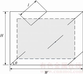
Figure 4 Area including midpoints of contained traces
After calculating c(s), ��v could be calculated as follows:
 (7)
(7)
3.2 Estimation error contrast analysis
The principles of the 4 methods are very different. In order to estimate the accuracy of the four methods, Monte-Carlo simulation was used to evaluate and verify the applicability and accuracy of these methods. 10 predefined 3-D fracture network models with different fracture numbers (density) were built and each model had 2 fracture sets. In Set 1, the number of fractures varies from 2000 to 6500 with 500 as the step size, and the number of fractures in Set 2 varies from 4000 to 8500 with the same step size. Detailed geometry parameter values are available in Table 2. The model scale is a cube whose length is 40 m. In order to eliminate the uncertainty caused by the occurrence, the occurrence is set to a constant. Based on the location and diameter distributions, the corresponding parameters of each fracture were obtained by Monte-Carlo method, then the fracture network model could be built. Considering the sampling bias, in each pre-defined fracture model, the Monte-Carlo simulation was repeated 5 times, and in each simulation, 2 sampling windows were cut and extracted for estimation error contrast. So, there were 10 sets of estimation results in each model.
In view of the boundary effect of the model [25], which means if the size of sampling window is equal to the model boundary, when counting the number of different types of traces, as shown in Figure 5, some traces whose center point is out of the boundary but intersects with the boundary cannot be counted in type (b) traces actually. This is because all the centers of simulated fracture discs are in the model boundary. Affected by this, the estimation result will have deviation. So, the size of the sampling window was set to 35 m��35 m, which was smaller than the size of model boundary. The relative error (RE) was used to represent the error between the estimated volume density and the predefined volume density.
The mean RE was taken after 10 repeated tests at each model. Figure 6 shows the relative error variation of 4 different estimation methods in two sets. According to them, the following conclusions can be drawn: 1) when the fracture density is small (<0.15 m�C3), the estimation accuracy of the methods is not obviously related to the fracture volume density. But with the increasing of volume density, the number of traces in sampling window raised, and the relative error declined steady except the K-Wu method. 2) K-Wu method will lead to a larger error than the other 3 methods. And with the trace number increased, the relative error did not reduced. This may be due to the probabilities of trace midpoints within the window needing to be calculated, and the probabilities are related to trace length [4]; when the number of type (a) and type (b) traces raise, the estimation uncertainty of the area density become larger, which leads to a strong error fluctuation and low precision of fracture volume density. 3) According to Figure 6, the estimation error of the other three methods could be sorted by the following order: Song2006 method>Oda method>Mauldon method, and the estimation error of Mauldon method is generally less than Oda method and Song2006 method. Therefore, the fracture density estimation with Mauldon method has the optimal result among the four methods. Relative error varies from 1.53% to 13.06%. In this paper, Mauldon method is suggested to estimate the fracture volume density.
Table 2 Data of diameter and orientation

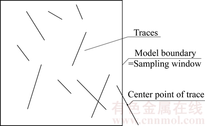
Figure 5 Schematic diagram of boundary effect

Figure 6 Relative error fluctuation of volume density in different method:
4 Error contrast of fracture size estimation methods
The fracture size estimation includes the ��forward modeling�� and the ��inverse modeling��. The ��forward modeling�� method may lead to a large computational cost. Therefore, four mainstream ��inverse modeling�� methods (Table 1) were adopted to estimate the fracture size distribution. And the estimation errors were compared.
4.1 Main principle of estimation methods
The first method was designated as the Einstein method [16].This method assumed that the coefficient of variation (COV) of the trace length distribution between finite window and infinite window is equal (considering the sampling bias). So, the standard deviation of trace length could be calculated after the mean trace length was estimated.
Based on Eq.(8), which is the stereological relationship between the true trace length distribution and the fracture diameter distribution [12], and assuming the diameter distribution form, the relationship of mean value and standard deviation between diameter and trace length can be derived:
 (8)
(8)
where g(D) is the density function of fracture diameter; m is the mean diameter; f(l) is the true trace length distribution in infinite window.
The Crofton��s theorem is then used to test and confirm the finally diameter distribution. Checking the equality of Eq.(9) corresponding to each assumed classical distribution form (lognormal, gamma, etc.) of D by trial method, the best distribution of D is the distribution for which the left and right sides are the closest to each other.
 (9)
(9)
where D is the fracture diameter; l is the trace length.
The second method is designated as the Song2001 method [13]. This method firstly built the equation between the true trace length distribution in infinite window and the trace length distribution with both ends observed:
 (10)
(10)
where f c(l) is the trace length distribution with both ends observed;  is the number of all type (c) traces within the window; ��A is the trace area density which can be calculated by Eq.(3).
Equation (8) was used to determine the fracture diameter distribution. Specific solution process can be obtained by the original paper.
The third method is designated as the Song2006 method [7]. The fracture diameter distribution could be estimated by the trace length histogram as shown in Eq. (5).Through discretizing Eq. (5), the diameter distribution can be calculated by solving an equation group.
The fourth method is designated as the Tonon method [14], which is similar to the Song2001 method. But in this method,Eq.(8) was transformed into an Abel integral equation by closed-form integral solution [26]:
 (11)
(11)
Numerical and closed-form solutions were applied into the fracture diameter estimations with the assumption of different trace length distribution forms.
4.2 Estimation error contrast analysis
For convenience, the predefined fracture network models for the estimation error contrast are the same as the models in Section 3.2. Lognormal distribution form for the diameter distribution was assumed in the predefined model and other distribution forms would not be studied in this work.
After obtaining the fracture diameter distribution by different methods, the area difference of P.D.F was defined as the sum of absolute values of the area difference at each division between the predefined distribution and the estimated distribution, which was treated as the composite error of the estimated distribution. For example, if the predefined and estimated distributions are not completely coincided in Figure 7, the area difference of P.D.F is the sum of the shaded area. Figure 8 shows the area difference of P.D.F with different methods. Then the lognormal distribution form was used to fit the estimation result in different methods and the relative error of mean diameter (REM) and the relative error of standard deviation of the diameter (RES) were calculated. Figure 9 shows the relative error of distributed parameters fluctuation in different methods.

Figure 7 Schematic diagram of area difference of P.D.F

Figure 8 Errors of four methods in estimation of diameter distribution:
The following conclusions can be drawn from comparative analysis: 1) From Figure 8, the error of the estimated distribution decreased with the increasing of fracture volume density. The error of the estimated distribution with the Einstein method or the Song2006 method is far less than the other two methods. 2) From the Figures 9(a) and (b), the REMs with Einstein method and Song2006 method are all less than 10%, which are better than the other two methods. The REM of four methods could be sorted by the following order: Tonon method>Song2001 method>Song2006 method> Einstein method. 3) Figures 9(c) and (d) show that the RESs with Einstein method and Song 2006 method are less than 50%, and the two methods have a stable downward trend with volume density increasing. In Set 1, the RES with Einstein or Song2006 method is greater than the RES with Song2001 or Tonon method; and in Set 2, the situation is quite the opposite. The RESs with Song2001 and Tonon method fluctuated greatly in two sets. The reason may be that the standard deviation estimations with Song2001 method and Tonon method are related to the fracture size magnitude and the occurrence. The Einstein method and Song2006 method can lead to more stable standard deviation results.
Therefore, the REM by Einstein method or Song2006 method is smaller and the RES is more stable. And with the consideration that the mean diameter is related not only to the fracture size estimation, but also to the fracture volume density (Eq. (2)), the Einstein method and the Song2006 method are suggested to estimate the fracture diameter distribution. Although the Einstein method seems to be more stable and accurate than the Song2006 method in Figures 8 and 9, the difference is not very big. And the Song2006 method is more simple and effective than the Einstein method in calculation principle, the computation of Song2006 method is much smaller and without trial process. On the other hand, Einstein method does not have universal applicability, the distribution form that is not classical or not used in trial method may be more accurate but can��t be tested and verified. And the assumption in Einstein Method that trace length distribution form was same in finite window and infinite window is not very reasonable [10, 14]. Therefore, the Song2006 method is selected in this paper for fracture size estimation.

Figure 9 Mean (a, b) and standard (c, d) relative error of four methods in estimation of diameter distribution:
5 3-D fracture network dynamic modeling method
When the fracture volume density estimation method and the fracture size distribution estimation method are confirmed, the 3-D fracture network model based on the Baecher disc model can be built. But there are some deviations between the model and the real geological fracture conditions. The traditional methods to check the deviation include graphical check and numerical examination. But the traditional methods are not systematic and few researchs focus on model accuracy improvement. In this section, the error index was created to characterize the deviation between the fracture network model and the measured data. And then the 3-D fracture network dynamic modeling method was built based on the downhill simplex method, in which the modeling input parameters (fracture density and diameter) were dynamically adjusted to reduce the error index of the model.
5.1 Calculation of fractal dimension in rectangular window
The fractal dimension of traces in rectangular window is usually calculated by box dimension. Assume that the traces are within a square window with side length L0; the window area is divided into (L0/l)2 boxes of which length is l; N(l) is the number of boxes containing traces or intersecting with traces (see Figure 10). Then change the box length l, a series of l-N(l) data can be obtained. Drawing logarithmic curve of N(l) and 1/l, the slope of the straight line (see Figure 11) is the fractal dimension.
As known that for the fractal dimension a close relationship exists with fracture parameters, the parameter can be treated as a quantitative value to represent the trace distribution and dispersion characteristics. Accordingly, it can be used for expressing the deviation between the fracture network model and the measured data.

Figure 10 Box method for solving fractal dimension

Figure 11 Fractal dimension calculation principle
5.2 Error index for model checking
Traditional ways for checking fracture network model error include graphical check and numerical examination. The graphical check means comparing the trace image in real sampling window with the trace image in the same direction window slit in the fracture network model and the reliability of the model could be judged qualitatively. The numerical examination means comparing the numerical characteristics between the real sampling window and the model sampling window, which includes mean trace length, mean occurrence, spherical deviation of occurrence, number of traces, etc. In the inverse modeling method [21], the relative error index which only includes the trace density and trace length was set up to express the fracture network model deviation:

 (12)
(12)
where n is the number of sets; i is the ith set; c and m respectively represent the prototype value and model value; u is the mean trace length; �� is the standard deviation of trace length; d is the line density of traces; p is the area density of traces.
Based on the aforementioned research, the model checking procedure was proposed and the error index was created and combined with fractal dimension. When the fracture network model was built, the graphical check method was firstly used to judge whether the model sampling window is similar to the real sampling window. Then the numerical examination was adopted:
1) The relative errors of the mean trace length, trace area density, mean occurrence, spherical deviation of occurrence, number of traces and fractal dimension were given:
 (13)
(13)
where M is the numerical characteristics in the model sampling window; F is the numerical characteristics in the real sampling window, when the relative error indexes are all less than 30%, the model can be used for further optimization; otherwise, re-simulating.
2) Considering that the dip and dip direction are correlated, the spherical deviation can be used to express the dispersity of the occurrence:
 (14)
(14)
 (15)
(15)
where f is the spherical deviation; N is the number of traces in one set; li, ni, mi are the ith components of normal vector of fracture disc. If f<0.25, the dispersity of the occurrence is acceptable, and the occurrence data are effective; otherwise, re-simulating.
After numerical examination passed, the error index could be calculated. The error index was defined to represent the deviation between the 3-D fracture network model and the measured data based on the relative absolute error (RAE):

 (16)
(16)
where symbolic meaning is the same with the symbolic in Eq. (12); r is the fractal dimension in sampling window;  is the mean value among the mean trace lengths in n trace sets;
 and
and  have the same meaning.
The fractal dimension error calculation did not consider the fracture grouping and the traces within the window are all integrated to calculate the fractal dimension. So, the error of fractal dimension is calculated by relative error (RE). The other parameters errors were expressed by relative absolute error (RAE).
The RAE takes the total absolute error of the model value and prototype value in n sets, then is divided by the total absolute error of the prototype value and the mean prototype value in n sets. The model accuracy is increased with the reduction of the error index. If the RE is used to build the error index like the inverse modeling method, the error would be influenced by the measured value of the denominator and the RE value may not truly reflect the model deviation. The following examples will illustrate.
If only the trace area density is considered for the error index, and there are two fracture sets. The error index with RE can be expressed as follows:
 (17)
(17)
The error index with RAE can be expressed as follows:
 (18)
(18)
Two simulations have been done and the trace area densities in two model are shown in Table 3. In the first simulation, the deviation occurred in Set 1 with 0.1, and in the second simulation, the deviation occurred in Set 2 with 0.1. The accumulated trace area density deviations in two simulation is all 0.1, which means that the deviation of trace number in unit area in each set is equal, but the error index with RE is different, influenced by the order of magnitude of prototype density. And the error index with RAE is equal in two simulations. So, the RAE is better than RE for the error index.
Table 3 Effectiveness of relative error and relative absolute error

5.3 3-D fracture network dynamic modeling procedure
Based on the result of estimation error contrast analysis, the Mauldon method and the Song2006 method are selected for fracture density and diameter estimation. Then the 3-D fracture network modeling procedure can be confirmed, but the error of the fracture network model still cannot be accepted. Considering that the ultimate goal is making the model closer to the real fractures, it can be transformed into an optimization problem. The objective function is the minimum of error index (Eq. (16)), decision variables are the input parameters for modeling. It can be learned that the fracture volume density, fracture diameter and the occurrence distribution have a direct impact on the accuracy of the fracture network model. With overall consideration of the dimension of the search space and the importance of the decision variables, the fracture volume density, mean value and standard deviation of the diameter distribution were used to create the decision variables:
 (19)
(19)
where i means the ith set; Si is the correction coefficient of the fracture volume density; Ti is the correction coefficient of mean value of diameter distribution; Ci is the correction coefficient of standard deviation of diameter distribution; ui and ��i
are the mean value and standard deviation of diameter distribution by Song2006 method; Ui and �� i are the corrected values.
The correction coefficients can be used as the decision variables, and the downhill simplex method was used as the optimization algorithm, which was applied in inverse modeling method successfully [21]. The downhill simplex is a direct search algorithm for extreme value in multivariable function. This method is applicable to the system that the relationship between the objective function and the decision variables cannot be expressed by explicit mathematical formula. Besides, the initial values of the volume density and diameter distribution parameters estimated by the methods selected in Section 3, 4 would be more accurate, which is beneficial to get the optimum solution quickly and accurately.
On the basis of the error analysis, the 3-D fracture network dynamic modeling method can be built (see Figure 12). After statistical homogeneity zoning and dominant partitioning works, the traces in different set within sampling window are used to estimate the distributions of geometry parameters. Then Monte-Carlo simulation technique is used to simulate the fracture data sets. When the model is done, the validation of fracture network is tested by graphical check and numerical examination. If the numerical characteristics in model sampling window all meet the requirements in Section 5.2, the model can be used as initial model and further optimized by dynamic modeling method. Owing to uncertainty of random sampling, the sampling result by Monte-Carlo method is different in each simulation. Therefore, it is suggested that the optimal result of 5 simulations is selected for each iteration of the dynamic modeling process. In the dynamic modeling process, taking the error index as the objective function, the downhill simplex method is used to search the feasible region of the correction coefficients. When the error index reached to the algorithm stop condition: ��<��0, the 3-D fracture network model is outputted. And taking the convergence and computational cost of the algorithm into account, ��0 could be equal to 1/5�C1/10 of the initial error index.

Figure 12 Flowchart of dynamic modeling of 3-D fracture network in dam foundation
6 Engineering case verification
In this section, two curtain grouting units in Miao Wei hydropower project in Southwest China were chosen for the 3-D fracture network modeling. Two curtain grouting units were judged as a statistical homogeneity by Schmidt��s equal-area projection. The study region was 70 m��70 m��50 m (length��width��height). The length of sampling window in study region was 60 m,the width was 50 m and 215 traces were recorded in the window. The fractures were divided into 2 sets based on the occurrence.
The statistical results showed that the occurrence in Set 1 obeys Fisher distribution, and the occurrence in Set 2 obeys Bivariate normal distribution. The fracture volume density and diameter distribution were estimated by methods chosen in Sections 3 and 4. Figure 13 shows the comparison of fracture network between the measured window and simulation window. The sketch picture slit in the model is close to the real sampling window, but the trace lengths in Set 1 seem to be longer than the measured values. According to the numerical examination, the numerical characteristics all meet the standard.
On this basis, the downhill simplex method was used to optimize the mode. There are 2 fracture sets with 6 correction coefficients. So, the search space dimension is 6 and the objective function is the minimization of error index in Eq. (16). The stop condition is that when the error index was less than 1/7 of the initial error index, the model optimization is completed. Based on flowchart in Figure 12, and begining with the initial model, the error index is calculated. If the error index does not achieve the stop condition, then change values of the 6 correction coefficient by reflection, expansion, contractions or shrink strategies step in downhill simplex method. The fracture model could be built with new volume density and diameter distribution and the stop condition is tested again. After some iterations, the final model can be obtained. Table 4 shows the comparison between the initial geometry parameters and the optimized geometry parameters. Table 5 shows the numerical characteristics and error index comparison. The comparison tables show that the 3-D fracture network dynamic modeling method works well, and the error index is successfully converged to the default value. The model fits well with the measured data, which can provide a more accurate 3-D fracture network model in statistical sense. From the prospective of engineering, the model has contributed to analyzing the distribution law of fractures in the rock mass of dam foundation. In the meanwhile, the stability, grouting and seepage analysis can be carried on, which can help scholars to understand the permeability and hydraulic characteristics in rock mass, then realize the simulation and prediction of grouting [32]. Figure 14 shows the effect drawing of the final 3-D fracture network model.
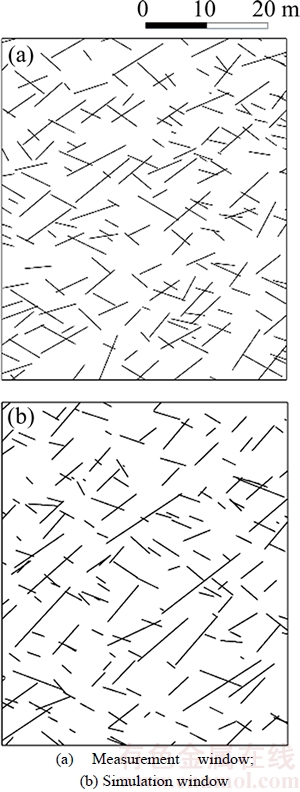
Figure 13 Sketch picture comparison of fracture network in exposed surface:
Table 4 Results of fracture parameters by optimization procedure

Table 5 Parameter comparison between optimized model and measured data in sampling window


Figure 14 Final 3-D fracture network model in rock mass of dam foundation
7 Conclusions
Accurate 3-D fracture network model is the basis of the mechanics and hydraulics analysis of dam foundation. In this paper, the 3-D fracture network dynamic modeling method focusing on the model error from the error of parameters estimation was built. The following conclusions can be drawn:
1) The mathematical model of 3-D fracture network dynamic simulation was proposed, which provides a research idea for reducing the uncertainty of 3-D fracture network model in rock mass of dam foundation.
2) In light of error contrast analysis of fracture size and density estimation methods in Section 3 and 4, the Mauldon method was selected for the fracture volume density estimation and the Song2006 method was selected for the fracture size estimation. Both of these 2 methods can get more accurate and stable estimation results.
3) Based on RAE, the error index was established to express the model deviation from measured data, and error index with RAE was proved to be more reasonable than the error index with RE. The fractal dimension was also applied in the error index which made the index more effective.
4) According to the above results, the 3-D fracture network dynamic modeling method was built by downhill simplex algorithm. Through repeated iteration, the initial values of fracture volume density and diameter distribution parameter are corrected to reduce the error index. Finally, the 3-D fracture network model can be obtained, which has little deviation from measured data in statistical significance.
5) The dynamic modeling method was verified using the data from a hydropower project in China that the error index reduced from 2.618 to 0.337, the numerical characteristics calculated by optimized model were generally close to those by measured data.
References
[1] BAECHER G B, LANNEY N A. Statistical description of rock properties and sampling [C]// Proceeding of the 18th US Symp Rock Mechanics (5C). Colorado: Golden, 1978: 1�C8.
[2] ZHOU Fu-jun, CHEN Jian-ping, NIU Cen-cen. Study of discontinuity density of fractured rock masses based on fractal theory [J]. Journal of Rock Mechanics & Engineering, 2013, 32(S1): 2624�C2631. (in Chinese)
[3] ODA M. Fabric tensor for discontinuous geological materials [J]. Journal of the Japanese Society of Soil Mechanics & Foundation Engineering, 1982, 22(4): 96�C108. DOI: https://doi.org/10.3208/sandf1972.22.4_96.
[4] KULATILAKE P H S W, WU T H. The density of discontinuity traces in sampling windows [J]. International Journal of Rock Mechanics & Mining Science & Geomechanics Abstracts, 1984, 21(6): 345�C347. DOI: http://dx.doi.org/10.1016/0148-9062(84)90367-X.
[5] MAULDON M. Estimating mean fracture trace length and density from observations in convex windows [J]. Rock Mechanics & Rock Engineering, 1998, 31(4): 201�C216. DOI: http://dx.doi.org/10.1007/s006030050021.
[6] WANG Liang-kui, CHEN Jian-ping, LU Bo. Estimation and application of volume density of discontinuities in sampling window [J]. Coal Geology & Exploration, 2002, 30(3): 42�C44. (in Chinese)
[7] SONG J J. Estimation of a joint diameter distribution by an implicit scheme and interpolation technique [J]. International Journal of Rock Mechanics & Mining Sciences, 2006, 43(4): 512�C519. DOI: http://dx.doi.org/10.1016/j.ijrmms.2005.09. 009.
[8] BARTH LMY J F, GUITON M L E, DANIEL J M. Estimates of fracture density and uncertainties from well data [J]. International Journal of Rock Mechanics & Mining Sciences, 2009, 46(3): 590�C603. DOI: 10.1016/j.ijrmms. 2005.09.009.
[9] JA'FARI A, KADKHODAIEILKHCHI A, SHARGHI Y, GHANAVATE K. Fracture density estimation from petro physical log data using the adaptive neuro-fuzzy inference system [J]. Journal of Geophysics & Engineering, 2012, 9(1): 105�C114. DOI: 10.1088/1742-2132/9/1/013.
[10] ZHU He-hua, ZUO Yu-long, LI Xiao-jun, ZHUANG Xiao-ying, DENG Jian. Estimation of the fracture diameter distributions using the maximum entropy principle [J]. International Journal of Rock Mechanics & Mining Sciences, 2014, 72(72): 127�C137. DOI: 10.1016/j.ijrmms. 2014.09.006.
[11] POINTE P R L, WALLMANN P C, DERSHOWITZ W S. Stochastic estimation of fracture size through simulated sampling [J]. International Journal of Rock Mechanics & Mining Science & Geomechanics Abstracts, 1993, 30(7): 1611�C1617. DOI: 10.1016/0148-9062(93)9-0165-A.
[12] WARBURTON P M. A stereological interpretation of joint trace data [J]. International Journal of Rock Mechanics & Mining Sciences & Geomechanics Abstracts, 1980, 17(4): 181�C190. DOI: 10.1016/0148-9062(80)910-84-0.
[13] SONG J J, LEE C I. Estimation of joint length distribution using window sampling [J]. International Journal of Rock Mechanics & Mining Sciences, 2001, 38(4): 519�C528. DOI: 10.1016/S1365-1609(01)00018-1.
[14] TONON F, CHEN S. Closed-form and numerical solutions for the probability distribution function of fracture diameters [J]. International Journal of Rock Mechanics & Mining Sciences, 2007, 44(3): 332�C350. DOI: 10.1016/j.ijrmms. 2006. 07.013.
[15] CROFTON M W. Probability [M]. 9th ed. Chicago: Encyclopedia Britannica Inc., 1885.
[16] ZHANG L, EINSTEIN H H. Estimating the intensity of rock discontinuities [J]. International Journal of Rock Mechanics & Mining Sciences, 2000, 37(5): 819�C837. DOI: 10.1016/S1365-1609(00)00022-8.
[17] HUANG Lei, TANG Hui-ming, ZHANG Long, CHENG Hao, ZUO Zong-xing, GE Yun-feng. Applicability of Priest-Zhang algorithm and revised algorithm for semi-trace line sampling to estimate rock discontinuities diameter [J]. Journal of Central South University: Science and Technology, 2012, 43(4): 1405�C1410. (in Chinese)
[18] WANG Shu-lin. Verification of random 3-D fractures network model of rock mass [J]. Journal of Engineering Geology, 2004, 12(2): 177�C181. (in Chinese)
[19] GUO Liang, LI Xiao-zhao, ZHOU Yang-yi, ZHANG Yang-song, SUO Pei-si, TU Chun-chun. Simulation of random 3d discontinuities network based on digitalization and its validation test [J]. Journal of Rock Mechanics & Engineering, 2015, 34(S1): 2854�C2861. (in Chinese).
[20] JIA Hong-biao, TANG Hui-ming, LIU You-rong, MA Shu-zhi. Theory and engineering application of 3-D network modeling of discontinuities in rock mass [M]. Beijing: Science Publishing House, 2008. (in Chinese)
[21] YU Qing-chun, OHNISHI Y. Three-dimensional discrete fracture network model and its inverse method [J]. Earth Science-Journal of China University of Geosciences, 2003, 28(5): 504�C522. (in Chinese)
[22] WANG Xiao-ming. Study on rock fractures and rock blocks in Wudongde dam area [D]. Beijing: China University of Geosciences (Beijing), 2013. (in Chinese)
[23] WU Qiong, KULATILAKE P H S W, TANG Hui-ming. Comparison of rock discontinuity mean trace length and density estimation methods using discontinuity data from an outcrop in Wenchuan area, China [J]. Computers & Geotechnics, 2011, 38(2): 258�C268. DOI: 10.1016/j.com- pgeo.2010.12.003.
[24] KARZULOVIC A, GOODMAN R E. Determination of principal joint frequencies [J]. International Journal of Rock Mechanics & Mining Science & Geomechanics Abstracts, 1985, 22(6): 471�C473. DOI: 10.1016/0148-9062(85)90012-9.
[25] LI Xiao-zhao, ZHOU Yang-yi, WANG Zhi-tao, ZHANG Yang-song, GUO Liang, WANG Yi-zhuang. Effect of measurement range on estimation of trace length of discontinuities [J]. Chinese Journal of Rock Mechanics & Engineering, 2011, 30(10): 2049�C2056. (in Chinese)
[26] L A. Incision or projections analysis about the distribution of corpuscles size contained in the body [J]. Statistics and Operation Researching, 1955, 6(3): 181�C196. (in Spanish) . DOI: 10.1007/BF03005853.
[27] MANDELBROT B B, AIZENMAN M. Fractals: Form, chance, and dimension [J]. Physics Today, 1979, 32(5): 65�C66. DOI: https://doi.org/10.1063/1.2995555.
[28] POINTE P R L. A method to characterize fracture density and connectivity through fractal geometry [J]. International Journal of Rock Mechanics & Mining Sciences & Geomechanics Abstracts, 1988, 25(6): 421�C429. DOI: 10.1016/0148-9062(88)90982-5.
[29] RONG Guan, ZHOU, Chuang-bing. Study on fractal dimension of discontinuity distributy based on simulation technique of discontinuity network [J]. Chinese Journal of Rock Mechanics & Engineering, 2004, 23(20): 3465�C3469. (in Chinese)
[30] LIU Bo, JIN Ai-bing, GAO Yong-tao, XIAO Shu. Construction method research on DFN model based on fractal geometry theory [J]. Rock and Soil Mechanics, 2016, 37(1): 625�C638. (in Chinese)
[31] PENG Kang, LI Xi-bing, WANG Ze-wei, LIU Ai-hua. A numerical simulation of seepage structure surface and its feasibility [J]. Journal of Central South University, 2013, 20(5): 1326�C1331. DOI: 10.1007/s11771-013-1619-3.
[32] YAN Fu-gen. Theories and applications of unified grouting model and analysis in hydraulic and hydroelectric projects [D]. Tianjin: Tianjin University, 2014. (in Chinese)
(Edited by YANG Hua)
���ĵ���
������������ˮ�繤�̰ӻ�������ά��϶���綯̬ģ���о�
ժҪ����Ӱӻ�������϶��ˮ�繤�̰��尲ȫ���ȶ���Ӱ�����ȷ�İӻ�������ά��϶����ģ���ǰӻ��ȶ����ཬ�����������Ļ����������о���ע�ض���϶���β���(�ߴ硢��״��λ�á��ܶ�)���о������Ʒ��������ڶ࣬�Ҵ������˸���������Լ��Բ������Ƶľ��ȣ�ȱ���о���϶ģ�;��ȼ�����ģ��ȷ�Եķ���������������⣬�������������Խ���ģ����ʵ������ƫ�����ģ��ȷ��ΪĿ�ģ����������������ˮ�繤�̰ӻ�������ά��϶���綯̬��ģ���������ȣ���4λѧ��(ODA, KULATILAKE, MAULDON��SONG)��������ܶȹ��Ʒ����Լ���3λѧ��(EINSTEIN, SONG, TONON)�����������϶�ߴ���Ʒ����������жԱȷ�������ȷ�����ŵIJ������Ʒ�������Σ��������ά����������Ծ�����������ģ����ʵ������ƫ������ָ�ꣻ����������ɹ���������ά��϶���綯̬��ģ����������С�����ָ��ΪĿ�꺯����������ɽ�����η���̬������϶���ܶȼ�ֱ��������ʼֵ������ģ�����ָ�꣬���յõ�ͳ�������Ϸ���Ҫ�����ά��϶����ģ�͡����÷���Ӧ����ijˮ�繤�̰ӻ���ά��϶ģ���У������������ά��϶����ģ�;��Ƚϸߣ���ʵ�����ݵ���ϳ̶ȸߡ�
�ؼ��ʣ�ˮ�繤�̰ӻ����壻��ά��϶���綯̬ģ�⣻����ά��������������Ծ�������ɽ�����η�
Foundation item: Project(51321065) supported by the Innovative Research Groups of the National Natural Science Foundation of China; Project(2013CB035904) supported by the National Basic Research Program of China (973 Program); Project(51439005) supported by the National Natural Science Foundation of China
Received date: 2016-08-30; Accepted date: 2018-01-20
Corresponding author: WU Bin-ping, PhD, Lecturer; Tel: +86�C15022400609; E-mail: wubinping@tju.edu.cn; ORCID: 0000-0002- 9398-9078

