J. Cent. South Univ. (2012) 19: 1148-1154
DOI: 10.1007/s11771-012-1121-3
An improved adaptive response surface method for
structural reliability analysis
LIU Ji(刘霁)1, 2, LI Yun(李云)2
1. School of Civil Engineering and Mechanics, Central South University of Forestry and Technology,Changsha 410004, China;
2. College of Civil Engineering, Hunan City University, Yiyang 413000, China
? Central South University Press and Springer-Verlag Berlin Heidelberg 2012
Abstract: The response surface method (RSM) is one of the main approaches for analyzing reliability problems with implicit performance functions. An improved adaptive RSM based on uniform design (UD) and double weighted regression (DWR) was presented. In the proposed method, the basic principle of the iteratively adaptive response surface method is applied. Uniform design is used to sample the fitting points. And a double weighted regression system considering the distances from the fitting points to the limit state surface and to the estimated design points is set to determine the coefficients of the response surface model. Compared with the conventional approaches, the fitting points selected by UD are more representative, and a better approximation in the key region is also observed with DWR. Numerical examples show that the proposed method has good convergent capability and computational accuracy.
Key words: response surface; structural reliability; uniform design; weighted regression
1 Introduction
Structural reliability analysis is a logical extension of conventional deterministic analysis, in which the inherent stochastic uncertainties of input parameters (such as loads, geometries and material properties) and/or computational modes are taken into account. Thus, it is regarded as a more rational safety evaluation and design theory for structures. In general, the fundamental issue of structural reliability involves the calculation of the failure probability, which could be defined as [1]
 (1)
(1)
where  is the vector of basic random variables;
  is the joint probability density function of the basic random variables; and
  is the limit state function which divides the space of basic variables into a safe domain
  and a failure domain F=
  The computational challenge of Pf lies in the determination of the limit state function
  which is usually highly nonlinear and very hard to obtain explicitly, especially in complex structural problems like
complicated structure system or time-variant system reliability analysis. In order to solve this kind of problems, several strategies including implicit first order reliability method (IFORM), Monte Carlo simulation (MCS) and response surface method (RSM) have been presented.
Generally, response surface method is a useful collection of mathematical and statistical technique for modeling and analyzing problems in which an interesting response is influenced by several variables and the objective is to optimize this response [2-3]. In the stage of RSM formation, its application is mainly focused on the fields of chemical and industrial engineering [4]. In the early stage of 1980s, the principle of RSM was introduced into the evaluation of structural reliability. The early literatures include HUANG and KOU [5] and GAYTON et al [6-7]. Then, the basic framework of the iteratively adaptive procedure was established by BUCHER and BOURGRUND [8], RAJASHEKHAR and ELLINGWOOD [9]. Based on this framework, a lot of researches and improvements have been performed on the selection of approximated response surface model, design of experiments (DOE) and estimation of undermined parameters. The first order polynomial [10-11], the second order polynomial [8-9, 12], the high order polynomial [13], the rational polynomial [14], the artificial neural network (ANN) [15-16], the radial basis function (RBF) [17] and the kriging [18] are selected as the approximated models. The 2k factorial design [19], the central composite design [19], the spherical 3k design [13] and the adaptive experimental design [20] are used to sample the fitting points. The interpolation technique [8, 12], the regression analysis [19], the weighted regression analysis [11, 20] and the moving least square [4] are utilized to evaluate the undetermined parameters.
The above-mentioned framework of adaptive response surface method was improved by using uniform design and double weighted regression. In the proposed method, the quadratic polynomial without cross terms is chosen as approximated function, and the uniform design is used to sample the fitting points. Then, a double weighted regression system considering the distances from the fitting points to the limit state surface and to the estimated design points is set to determine the coefficients of the approximated function.
2 Method
The basic principle of the RSM for structural reliability analysis is to use a simple function to approximate the performance function of structures. Based on this simple approximate function, the reliability index and failure probability can be evaluated easily using general reliability method like FORM. But the performance functions are usually very complex and every approximate function has its own rigidity. Thus, it is impossible to assure the accuracy of the approximation in the entire space of design variables. Therefore, if we simply follow the basic principle, it is impossible to gain accurate result. To overcome this issue, an iteratively adaptive procedure is suggested [8-13, 20]. As we know, the R-F reliability index β is defined as the distance from the origin to the design point in the standard design space. β would be obtained as soon as the design point is found. Therefore, instead of trying to approximate in the entire design space, the adaptive procedure seeks for the design point and manages to approximate exactly in the region by iteratively reconstructing the response model. The adaptive RSM involves the selection of approximate model, the choice of DOE, and the approach to determine the coefficients. The uniform design would be used to sample the design points and a double weighted system would be set to estimate the coefficients.
2.1 Uniform design
The uniform design is a new experimental design method developed by FANG [21]. It only considers the uniform distribution of experimental points in the design space. In the case that the factors and levels are the same, the number of experiments would be the least, equal to the maximum level of the factors. Taking the experiment with x factors and n levels for example, the number of experimental points is only equals to n, so that the experimental expense is sharply reduced. Furthermore, uniform design aims at arranging the experimental points in the design space uniformly. Any combinations of experiments would be controlled effectively. Consequently, the uniform design is extremely suitable for experiments with huge number of factors and levels, and the number of it is also constrained.
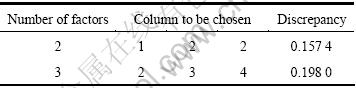
For convenient use of uniform design (UD), the uniform design tables (UDT),  or Un(nm), are developed to arrange the experimental points, where U stands for the uniform design, n is the number of levels which is equal to the number of experiments and m is the maximum number of factors arranged using tables. The UDT with a “*” in the top right corner has better uniformity and should be chosen for design as a priority. The discrepancy is used to weight the uniformity of UD. The less the discrepancy is, the more uniform the UD would be. So, the UDT with “*” is more uniform. The columns of UDT are not equal, and the columns to be chosen for a design are closely relevant to the number of the factors. Thus, every UDT has an accessory table for the selection of columns. In general, there are more than one UDT for experiments with determinated number of factors. As a result, a UDT which can meet the requirements of the experimental factors with small discrepancy and less experiments should be chosen. Table 1 gives the UDT
  and Table 2 gives its accessory table. They will be used in the numerical cases in the following section.
In the RSM, approximate models were fitted based on the experimental points sampled by a certain sort of DOE. The quality of DOE intensively affects the quality of the approximation, and then further affects the search of the design point and the evaluation of the reliability index. In the case of same number of experimental points, the UD could make the experimental points distribute in the design space as uniformly as possible. This would thoroughly benefit the construction of the approximate model. Thus, UD was chosen as the sampling method in this work. The steps to utilize the UD in the proposed method are as follows:
Table 1 UDT 
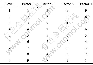
Table 2 Accessory table of UDT
1) Determine the sampling center of UD. Usually, the mean point is selected for the first step of iteration and for other steps, the sampling centers are determined according to Eq. (9).
2) Determine the radius of sampling by fiσi (i=1, …, n), where σi is the standard deviation of basic random variables, fi are assigned to be 2-3 for the first step, and 0.1-0.2 for other steps.
3) Determine the number of experimental points according to the number of coefficients to be determined in the approximate model.
4) Divide the sampling region into several levels according to the number of experimental points.
5) Select the UDT with the least discrepancy to arrange the experiments according to the number of factors and levels.
2.2 Double weighted regression
Conventionally, the coefficients of the approximate response functions are estimated by the least square method. That is, the coefficient vector A is gained by resolving the following linear system:
 (2)
(2)
where  is the vector of the values of performance function at the p different experimental points and M is the design matrix which is given by the p points of DOE:
In the case of a linear response model,
 (3)
(3)
In the case of a quadratic response model without cross terms, with i, j={i, …, n} and i≠j,
 (4)
(4)
In fact, equal weights are imposed on the p different sampling points in the above procedure. But it is not absolutely rational, because the objective of constructing the approximate function in the adaptive RSM is to seek for the design point. The sampling points which are closer to the limit state surface and design points should be given greater weights, so that the key region around this place would be better approximated. Therefore, a double weighted system is set as follows [20]:
 (5)
(5)
where Wk is the diagonal matrix of weight factors, of which the elements in the diagonal is the weight factors wk=wgkwdk imposed on different experimental points, and
 (6)
(6)
where g(xk) is the value of performance function at the k-th sampling point and g(x0) is the value of performance function at the mean point.
 (7)
(7)
where dk is the distance between the k-th point and the approximate design point obtained by the previous step of iteration in the standard space.
As shown in Eq. (6), greater weights are assigned to the sampling points at which the values of performance function are larger so that the region closer to limit state function will be fitted better. And the weight factors defined by Eq. (7) penalize the sampling points far from design point and make the region closer to the design point fitted better. By setting the double weighted system using wgk and wdk, the response will be approximated better in the key region and the accuracy and convergence capability of the proposed method will be improved as well.
2.3 Procedures of proposed method
The proposed method follows the framework of the adaptive RSM and uses the most popular pure quadratic polynomial without cross terms as the approximate function:
 (8)
(8)
The UD is used to sample the experimental points. The interpolation technique proposed by BUCHER and BOURGRUND [9] is used to determine the sampling center:
 (9)
(9)
The double weighted regression technique described in Section 2.2 is used to estimate the coefficients. And after an approximate model is built, the R-F method or an optimization method will be applied to obtain the reliability index and design point. The specific algorithm is as follows:
1) Postulate an initial iterative point 
 (usually select mean point).
2) Apply the UD to sample the fitting points according to the steps given in Section 2.1 and form a design matrix MK like Eq. (4), in which the subscript K denotes the time of iteration.
3) Compute the value of the performance function at the fitting points using FEM and generate the column vector 
4) Compute the weight factors wgk and wdk according to Eqs. (6) and (7). Then, estimate the coefficients a, bi, ci (i=1, 2, …, n) of Eq. (8) using Eq. (5).
5) Utilize the R-F method or the optimization method to resolve the design point and the reliability index, after the approximate model is gained by Step 4).
6) Check the convergence criterion |β(K)-β(K-1)|<ε, where ε is the accuracy specified by the user. If the criterion is satisfied, calculate the failure probability using Pf=Φ(-β(K)). Otherwise, return to Step 2) and begin the next step of iteration.
3 Numerical examples
3.1 Example 1
A simple example with two normally distributed random variables is used. The limit state function of the serviceability of a cantilever beam is:  0.018 461 54-74.769 23x1/
 and the random variables are independent, x1~N(1 000, 200) kN and x2~N(250, 37.5) mm.
This problem has an explicit limit state function and can be resolved by directly using R-F method. The results obtained by the R-F method, the method in Ref. [12] and the proposed method are lsited in Table 3. The UDT and were separately used to arrange experiments in the proposed method (7p) and proposed method (9p). As given in Table 3, the reliability index from Ref. [12] converges to 2.332 8 after five iterations. A total of 29
 were performed. The reliability index by the proposed method (7p) converges to 2.330 6 through four iterations. A total of 31 were performed. As the experiment arranged by is more uniform than the one arranged by
  the result by the proposed method (9p) converges more accurately to 2.330 9. In contrast to the method from Ref. [12], the proposed method converges faster and obtains more precise result. Figure 1 shows the convergence process of the proposed method (9p). As can be seen in Fig. 1, the proposed method converges fast to the exact design point and the response surface model approximates the true limit state surface well in the key region.
3.2 Example 2
The limit state function for structural reliability analysis is  in which the random variables are also independent, where x1~N(10, 5) and x2~N(9.9, 5).
As shown in Fig. 2, the limit state surface is extremely highly non-linear in the region around the design point and the constructed response surface model fits quite well in this region. Table 4 presents the results by the adaptive MCS, the direct optimization method and the proposed method (7p). The R-F method could not converge in this problem. The proposed method (7p) uses the optimization method to search the design point and yields to a reliability of 2.292 3. It is rather close to the result using the optimization method directly on the true limit state function. These results imply that the scheme of experiment design and the double weighted system is applicable to the highly non-linear problems. And the computational error is influenced by the method using for the search of the design point.
3.3 Example 3
The limit state function for structural reliability analysis is: g=YS-M, where random variables are independent, Y~LN (275.52, 34.44) MPa, S~LN (8.19× 10⁻⁴, 4.1×10⁻⁵) m3 and M~Type I Largest (1.13×10⁵, 2.26×10⁵) N・m.
Table 3 Proposed method of Example 1
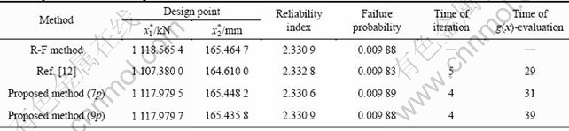
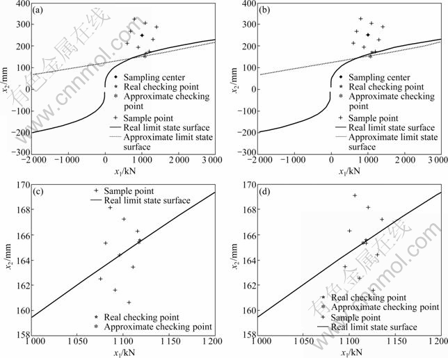
Fig. 1 Iterative convergence condition of Case 1 (proposed method (9p)): (a) First iterative step; (b) Second iterative step; (c) Third iterative step; (d) Fourth iterative step
Table 4 Proposed method of Example 2
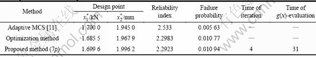
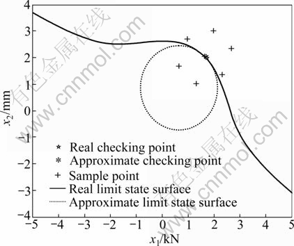
Fig. 2 Response surface function and design point of Example 2 obtained by proposed method
The random variables in this case are non-normally distributed. The equivalent procedure proposed by Rackwit and Fiessler was used to treat the non-normality of variables. The results of different methods are comparable (see Table 5). But the projection procedure proposed by Ref. [10] is tedious and needs more computational cost. The proposed method (7p) yields to a precise result after three steps of iteration.
3.4 Example 4
This example shows a steel joint with rising temperature and in the fatigue condition. The limit state function is strongly nonlinear and expressed as
 (10)
(10)
The random variables are independent and their distributions are listed in Table 6.
Table 5 Proposed method of Example 3
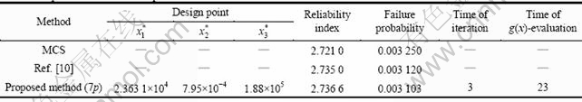
Table 6 Distributions of random variables in Example 4
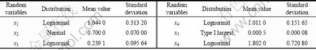
Table 7 Proposed method of Example 4
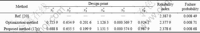
This case is a complex problem with six non-normally distributed variables and a strong nonlinear limit state function. It can be used to check the adaptability of the proposed method in complex problems. The results are given in Table 7. The uniform design table U17(178) was used in this case. The result of the proposed method was compared with the result from Ref. [20]. But, its adaptive DOE needs a procedure of coordinate selection based on derivation, nevertheless, the UD is more easily to execute.
4 Conclusions
1) An improved adaptive response surface method for complex structural reliability analysis with implicit limit state function is studied. The main characteristic of the improved method is that the UD is used to replace the traditional experimental design method to sample the fitting points and a named double weighted system is set to determine the coefficients of the response model. The double weighted system considers the influence of the distances from the fitting points to the limit state surface and to the estimated design point. The coefficients of response model determined by DWR are more rational.
2) The numerical examples show that the proposed method has good convergent capability and computational accuracy. Nevertheless, some drawbacks still exist. The computational accuracy is still dependent on the design point searching method. The uniformity of UD and the value of fi will affect the computational result. More research should be performed to uncover and quantify the influence, thereby, to guide the use of the proposed method.
References
[1] QIN Q L, LING D J, MEI Q. Theory and applications-reliability stochastic finite element methods [M]. Beijing: Tsinghua University Press, 2006: 73-92.
[2] KAYMAZ I, MCMAHON C A. A response surface method based on weighted regression for structural reliability analysis [J]. Probabilistic Engineering Mechanics, 2004, 20: 1-7.
[3] DUPRAT F, SELLIER A. Probabilistic approach to corrosion risk due to carbonation via an adaptive response surface method [J]. Probabilistic Engineering Mechanics, 2006, 21: 207-216.
[4] BUCHER C, MOST T. A comparison of approximate response functions in structural analysis [J]. Probabilistic Engineering Mechanics, 2008, 23: 154-163.
[5] HUANG S, KOU X J. An extended stochastic response surface method for random field problems [J]. Acta Mech Sin, 2007, 23: 445-450.
[6] GAYTON N, BOURINET J M, LEMAIRE M. CQ2RS: A new statistical approach to the response surface method for reliability analysis [J]. Structural Safety, 2003, 25: 99-121.
[7] GAVIN H P, YAU S C. High-order limit state functions in the response surface method for structural reliability analysis [J]. Structural Safety, 2008, 30(30): 79-162.
[8] BUCHER C G, BOURGRUND U. A fast and efficient response surface approach for structural reliability problems [J]. Structural Safety, 1990, 7: 57-66.
[9] RAJASHEKHAR M R, ELLINGWOOD B R. A new look at response surface approach for reliability [J]. Structural Safety, 1993, 12: 205-220.
[10] KIM S H, NA S. Response surface method using vector projected sampling points [J]. Structural Safety, 1997, 19: 3-19.
[11] ZHAO Y G, TETSURO O. Moment methods for structural reliability [J]. Structural Safety, 2001, 23: 47-75.
[12] TONG X L, ZHAO G F. The response surface method in conjunction with geometric method in structural reliability analysis [J]. Journal of Civil Engineering, 1997, 30(4): 51-57.
[13] GAVIN H P, YAU S C. High-order limit state function in the response surface method for structural reliability analysis [J]. Structural Safety, 2008, 30: 162-179.
[14] CHOWDHURY R N, XU D W. Rational polynomial technique in slope reliability analysis [J]. Journal of Geotechnical Engineering ASCE, 1993, 119(12): 1910-1928.
[15] DENG J, GU D S. Structural reliability analysis for implicit performance functions using artificial neural network [J]. Structural Safety, 2005, 27: 25-48.
[16] JIN C. A new artificial neural network-based response surface method for structural reliability analysis [J]. Probabilistic Engineering Mechanics, 2008, 23: 51-63.
[17] DENG J. Structural reliability analysis for implicit performance function using radial basis functions network [J]. International Journal of Solids and Structures, 2006, 43: 3255-3291.
[18] KAYMAZ I. Application of Kriging method to structural reliability problems [J]. Structural Safety, 2005, 27: 133-151.
[19] FARAVELLI L. Response-surface approach for reliability analysis [J]. Journal of Engineering Mechanics, ASCE, 1989, 115: 2763-2781.
[20] ZHOU H L, WU J G, WANG H J. Reliability analysis of response surface method based on a double weighted regression technique [J]. Journal of Zhejiang University of Technology, 2010, 38(2): 218-221.
[21] FANG K T. Uniform design and uniform design table [M]. Beijing: Science Press, 1994: 16-39.
(Edited by HE Yun-bin)
Foundation item: Project(50774095) supported by the National Natural Science Foundation of China; Project(200449) supported by National Outstanding Doctoral Dissertations Special Funds of China
Received date: 2011-01-04; Accepted date: 2011-05-20
Corresponding author: LI Yun, Associate Professor, PhD; Tel/Fax: +86-731-88877859; E-mail: liyunliuji@163.com

