J. Cent. South Univ. (2016) 23: 2453-2464

DOI: 10.1007/s11771-016-3304-9

Real-time road traffic states estimation based on kernel-KNN matching of road traffic spatial characteristics

XU Dong-wei(徐东伟)¹, WANG Yong-dong(王永东)¹, JIA Li-min(贾利民)²,

ZHANG Gui-jun(张贵军)¹, GUO Hai-feng(郭海锋)¹

1. College of Information Engineering, Zhejiang University of Technology, Hangzhou 310023, China;

2. State Key Laboratory of Rail Traffic Control and Safety (Beijing Jiaotong University), Beijing 100044, China

Central South University Press and Springer-Verlag Berlin Heidelberg 2016

Abstract: The accurate estimation of road traffic states can provide decision making for travelers and traffic managers. In this work, an algorithm based on kernel-k nearest neighbor (KNN) matching of road traffic spatial characteristics is presented to estimate road traffic states. Firstly, the representative road traffic state data were extracted to establish the reference sequences of road traffic running characteristics (RSRTRC). Secondly, the spatial road traffic state data sequence was selected and the kernel function was constructed, with which the spatial road traffic data sequence could be mapped into a high dimensional feature space. Thirdly, the referenced and current spatial road traffic data sequences were extracted and the Euclidean distances in the feature space between them were obtained. Finally, the road traffic states were estimated from weighted averages of the selected k road traffic states, which corresponded to the nearest Euclidean distances. Several typical links in Beijing were adopted for case studies. The final results of the experiments show that the accuracy of this algorithm for estimating speed and volume is 95.27% and 91.32% respectively, which prove that this road traffic states estimation approach based on kernel-KNN matching of road traffic spatial characteristics is feasible and can achieve a high accuracy.

Key words: road traffic; kernel function; k nearest neighbor (KNN); state estimation; spatial characteristics

1 Introduction

With the increasing demands of trip and transportation, the traffic problems such as traffic congestion and traffic safety are more and more prominent. This seriously affects the economic development and people’s life. The accurate acquisition of road traffic states is the most important and basic work in solving these traffic problems. For example, the traffic control and management system requires sufficient road traffic state data to generate appropriate traffic control strategies. The quality of traffic service also depends on the quality of the collected road traffic state information.

With the development of the information’s automation and intelligence, different kinds of detection devices have been used in the acquisition of road traffic states in succession. Although the traffic state detection technology has been developing day by day, the problems with traffic data, such as data invalidation and data loss, still occur frequently. So, the scenarios of long sequences of data loss in time and space series are frequently met in the collection of the road traffic state data. For example, the effective percentage of volume data collected by loop detectors in Beijing is only 24.02% from 2011-09-19 to 2011-09-23 [1]. This situation is mainly caused by a bug in the detectors’ capability, noise interference, communication failure, influences of the environment, and so on.

In this case, the historical imputation method is frequently used. The historical imputation method means to fill the missing data points with known road traffic state data collected from temporal-neighbouring (collected from the same sensor during the same period but in neighbouring days) or pattern-neighbouring (collected from the same sensor during the same period but in other days with similar road traffic running states) [2-3]. A variation of this algorithm is to fill the missing data points with the weighted road traffic state values collected within recent days. In addition, various imputation methods have also been explored for the road traffic states measurement for this case. HAWORTH and CHENG [4] presented a non-parametric spatio-temporal kernel regression method using the current traffic patterns of the upstream and downstream neighbouring links to forecast the future unit journey time values of road links in central London. RAY and DOUGLAS [5] proposed an empirical orthogonal functions to reconstruction historical sea level from the relatively sparse tide-gauge network. QU et al [6] put forward a probabilistic principal component analysis method to impute the missing flow volume data based on historical data mining, which reduced the root-mean-square by at least 25% than conventional methods. There are also other methods investigated in recent years, such as expectation maximization [7-8], dynamic graphical model [9], states space neural network [10], road traffic information templates [11], matching of the regional traffic attractors [12], compressive sensing [13], and so on.

With the increasing quality of collected road traffic state data, it is generally believed that more data help to build better road traffic states estimation models. But the parameter models cannot effectively reflect the complete characteristics of road traffic big data. Otherwise, the parameter models usually have many restrictions, which leads that it is difficult to realize all-purpose road traffic states estimation with them. The non-parametric models are mainly established based on road traffic data. The range of the general assumptions for non-parametric models is also very wide. So, the non-parametric models have better robustness and adaptability in the road traffic states estimation. But most of the existing algorithms based on non-parametric models for road traffic states estimation don’t take the multi-dimensional and multi- granularity characteristics of road traffic states into consideration.

The main problems discussed in this work are how to effectively estimate the road traffic data when large quantities of traffic flow data in time sequences are invalid and the traffic data of adjacent links are not always available. The road traffic running states have regularity and reproducibility property when the road condition and traffic flow condition are both similar [14-15]. So, under this situation, the historical road traffic state data can be used for traffic data imputation. But the road transportation system also has complexity and variability property, so its running states have certain randomness. The simple use of the historical traffic data for traffic data imputation cannot effectively reflect the real-time changes of road traffic running states.

Therefore a traffic states estimation algorithm based on kernel-KNN matching of road traffic spatial characteristics is proposed in this work. Through mapping the multi-dimensional and multi-granularity spatial road traffic state data into high dimensional feature space with the kernel function, the accurate acquisition of road traffic states can be realized.

2 Framework of algorithm

The change of road traffic states has regularity and reproducibility property. So, the road traffic states can be effectively estimated based on the effective matching of current and historical spatial road traffic states. Firstly, the representative road traffic state data are extracted to establish the RSRTRC. Then, the spatial road traffic state data sequences are selected to construct the kernel function. The relevant parameters can be determined by the training data set. Finally, the current and referenced spatial road traffic data sequences are obtained and mapped into high dimensional space. Through the selection of KNN, the road traffic states can be estimated. The algorithm framework is shown in Fig. 1.

3 Basic concept and principle of kernel function

Road traffic state can be represented by multi-dimensional parameters in time and space. Based on the regularity of road traffic states, the reappearance of road traffic states can be realized by pattern classification and identification. But the classification of multi-dimensional road traffic state data is a non-linear classification problem. So, the kernel function is introduced in this work. Through non-linear transformation, the multi-dimensional road traffic state parameters can become linearly separable by kernel function. Finally, the effective classification and identification of road traffic states can be realized.

Fig. 1 Framework of algorithm

Through non-linear transformation, kernel function can effectively solve the non-separable problems. The basic idea is to make original samples linearly separable in a new high dimensional feature space through kernel transformation. Then, the seeking of optimal classification can be achieved in the high dimensional feature space. The kernel function can reflect the similarity between two input data sets.

The definition of kernel function is shown as

K(x,z)=<φ(x), φ(z)>                           (1)

where x, z∈X; X∈Rⁿ; φ is a nonlinear function, which mappings the original samples space X into the high dimensional feature space H; H∈R^m; m< represents the scalar product.

The kernel function transforms the scalar product in the original samples space into the calculation of the kernel function in the high dimensional feature space. Any function satisfying the Mercer theorem can be taken as the kernel function. The Mercer theorem describes the property of kernel function, which is defined as follows:

For any symmetric function K(x, z), the necessary and sufficient condition that it is the scalar product in certain space is: for arbitrary φ(x), which is not identical to zero and, there will constant be

                     (2)

The use of kernel function provides a powerful and reasonable method for checking non-linear relationships with well-known linear algorithm. This method separates the algorithm design from description of the original feature space. So, it can avoid problems, such as confirming the form and parameters of nonlinear mapping functions, estimating the dimensions of feature space, and so on. The kernel function lays theoretical foundation for solving complicated classification or regression problems in high dimensional feature space.

4 Established RSRTRC

The road traffic states have regularity and repeatability property [16]. So, the reference sequences of road traffic running characteristics (RSRTRC) should be established first for estimating road traffic states. The establishment steps of RSRTRC can be summarized as follows.

1) Format design of RSRTRC

Let △t denote the collection interval of road traffic sates data. Then the time format of RSRTRC can be shown as follows.

The table format for the content and description of RSRTRC are defined as listed in Tables 1 and 2.

Fig. 2 Time format of RSRTRC

Table 1 Table format of content of RSRTRC

Table 2 Table format of description of RSRTRC

In Table 1, S_ta(t) is the link’s traffic states at time t, such as volume, occupancy, speed, time headway, and so on.

2) Data extraction and establishment of RSRTRC

Let r denote the number of the links having available traffic states data and spatial correlation with the target link, which are denoted as R₁, R₂…R_r, respectively. The representative historical traffic states data (b days) of (r+1) links are abstracted and preprocessed (mainly for some individual abnormal and missing traffic data). The preprocessed traffic states data are input into the RSRTRC. Finally, the RSRTRC are obtained.

5 Road traffic states estimation approach based on kernel-KNN matching of road traffic spatial characteristics

5.1 Construction of kernel function of spatial road traffic data sequence

Single road traffic parameter cannot effectively reflect the road traffic states. So, the road traffic states estimation approach based on the analysis of a single road traffic parameter has too many deviations and randomness. So, multi-dimensional and multi-granularity road traffic state data are used to estimate the road traffic states in this work.

Let △t denote the data collection interval of road traffic sensors. Let N_um denote the number of the data collected from one road traffic sensor every day. Let c×△t denote the selected time length. Let d denote the selected number of road traffic state parameters. Let r denote the number of the links having spatial correlation with the target link. Then, the selected spatial road traffic data sequence at time t is denoted as

X(t)=[S₁(t-(c-1)△t) …S₁(t-△t) S₁(t)

S₂(t-(c-1)△t) …S₂(t-△t) S₂(t)^T           (3)

…S_r(t-(c-1)△t) … S_r(t-△t) S_r(t)]

S_j(t)=[S_j1(t) S_j2(t) … S_jd(t)]^T              (4)

where S_j(t) is the road traffic state parameters on the jth link at time t; S_ji(t) is the value of ith road traffic state parameter on the jth link over [t, t+△t]; i=1, 2, …, d.

Suppose that the spatial road traffic data sequence X(t) is mapped into the high dimensional feature space by certain nonlinear mapping Then the scalar product of spatial road traffic data sequences in the high dimensional feature space at time t₁ and t₂ can be expressed by the kernel function as

        (5)

where the nonlinear mapping is determined by the expression form of the kernel function.

5.2 Estimation of road traffic states based on kernel-KNN matching of road traffic spatial characteristics

5.2.1 Selection of different spatial road traffic data sequences

In the process of estimating road traffic states based on kernel-KNN matching of road traffic spatial characteristics, there are mainly two relevant data sets: the referenced spatial road traffic data sequence and the current spatial road traffic data sequence.

There are a totally of a days’ historical traffic states data selected to establish the RSRTRC. The total number of the road traffic state data in the RSRTRC is a×N_um. Let (h·△t) denote the time of the hth data in the RSRTRC. The referenced spatial road traffic data sequence at time (h·△t) is denoted as

X_S(h·△t)=[S₁(h·△t-(c-1)△t) … S₁(h·△t-△t) S₁(h·△t)

S₂(h·△t-(c-1)△t) … S₂(h·△t-△t) S₂(h·△t)

…

S_r(h·△t-(c-1)△t) … S_r(h·△t-△t) S_r(h·△t)]^T

(6)

S_j(h·△t)=[S_j1(h·△t) S_j2(h·△t) … S_jd(h·△t)]^T       (7)

where S_j(h·△t) is the referenced parameters set in the RSRTRC on the jth link at time (h·△t); S_ji(h·△t) is the value of ith reference parameter on the jth link over [h·△t,(h+1)△t] in the RSRTRC; i=1, 2, …d; c-1≤h≤ (a×N_um-1).

Let t_N denote the current time, then the current spatial road traffic data sequence can be denoted as

X(t_N)=[S₁(t_N-(c-1)△t) … S₁(t_N-△t) S₁(t_N)

S₂(t_N-(c-1)△t) … S₂(t_N-△t) S₂(t_N)

…

S_r(t_N-(c-1)△t) … S_r(t_N-△t) S_r(t_N)]^T                                   (8)

S_j(t_N)=[S_j1(t_N) S_j2(t_N) … S_jd(t_N)]^T                     (9)

5.2.2 Acquisition of Euclidean distance in high- dimensional feature space of spatial road traffic data sequences

The multi-dimensional and multi-granularity spatial road traffic data sequences are mapped into the high dimensional feature space through kernel function. This process enables similar samples closer and different samples farther. Based on the definition of the kernel function, multi-dimensional and multi-granularity spatial road traffic data sequences can be mapped into the So, the Euclidean distance of the referenced spatial road traffic data sequence X_S(h·△t) and the current spatial road traffic data sequence X(t_N) in the high dimensional feature space can be denoted as

             (10)

5.2.3 Acquisition of road traffic states of target link

1) Based on Eq. (10), the Euclidean distance between the referenced and current spatial road traffic data sequence in the high dimensional feature space can be calculated. The k referenced spatial road traffic data sequences according to the k nearest neighbors can be selected, which are denoted as X_S(g_i·△t) respectively (1≤i≤k, c-1≤g_i≤(a×N_um-1)).

2) From the RSRTRC, the target link’s road traffic states at time (g_i·△t) can be selected, which are denoted as S(g_i·△t).

3) Then the road traffic state at time t_N can be obtained through the following equation:

                      (11)

where μ_i is the weight value of the ith road traffic state, which is inversely proportional to the Euclidean distance between the referenced and the current spatial road traffic data sequences in the high dimensional feature space.

6 Case studies

6.1 Preparations

6.1.1 Acquisition of data

Some typical expressways in Beijing were adopted for the experiment’s verification and analysis. The concrete information of the selected links is listed in Table 3. The link (HI7036b, Capital Library to Andingmen Bridge) was selected as the target link for experiment verification.

All experiment data were obtained from microwave sensors. The speed and volume are the main parameters collected by microwave sensors, and these two parameters are both the representative parameters of road traffic states. So, the experiments focused on these two road traffic state parameters.

Table 3 Information of selected links for experiments

The historical data (2011-06-01—2011-06-14) were extracted to establish the RSRTRC. The road traffic state data collection interval △t is 2 min.

The historical data (2011-06-18) were extracted as the training data set to determine the algorithm parameters. The data (2011-06-19/2011-06-25/2011- 06-26) were extracted as the experiment data set to verify the algorithm.

6.1.2 Choice of kernel function

The frequently-used Mercer kernel functions mainly conclude: Linear kernel function, polynomial kernel function, Gauss kernel function, sigmoid kernel function, Fourier kernel function, and so on. In this work, the Gauss kernel function was chosen for experiments. The basic expression of Gauss kernel function is shown as

                           (12)

The Gauss kernel function is chosen based on the following two reasons.

1) The Gauss kernel function has the separable characteristics.

The separable characteristics means the ability that the feature transformation derived from the kernel function can make the given training samples linearly separable in the characteristics space. As long as the parameters are appropriate, the training samples can always be linearly separated when the Gauss kernel function is chosen as the kernel function. The separable characteristics of the Gauss kernel function is determined by its own properties [17]. The training samples can all be correctly separated when the σ in the Gauss kernel function is small enough [18].

2) The Gauss kernel function has the local characteristics.

The training samples can all be linearly separated when the σ in the Gauss kernel function is too small, but the results are prone to be over fitting. This makes the generalization characteristics of the Gauss kernel function worse. From the expression of the Gauss kernel function, we can see that the Gauss kernel function only has effect when the distance between different samples is not more than σ. When the distance between different samples is larger than σ, the value of the Gauss kernel function tends to zero.

6.1.3 Parameters determination

In the process of estimating road traffic states based on the Gauss kernel function, the relevant parameters mainly include: the value of (σ), the time length (c·△t), and the value of (k). For different road traffic state data sets, the optimal parameters should be different. So, the determination of parameters here is a rough analysis of the parameters’ impact on the road traffic states estimation algorithm.

As these parameters all have influences on the accuracy of the algorithm, the separate analysis of each parameter’s influence on the algorithm’s accuracy can’t ensure the algorithm’s optimization. So, the effects of these parameters on the road traffic states estimation algorithm should be taken in consideration at the same time.

The absolute error e is introduced as index for researching the optimal parameters:

           (13)

For different (σ, c, k), there should be corresponding e. So, the following equation should exist.

e=ω(σ, c, k)                 (14)

That means that there should be some distribution relation ω between (σ, c, k) and e. The process of determining parameters is seeking the (σ, c, k) corresponding to the minimum NMAE. Then, we can get the following model:

Min ω(σ, c, k)     (15)

where .

Finally, the determination of (σ, c, k) can be obtained through the analysis of historical road traffic state data.

6.1.4 Influence analysis of parameters of algorithm

To show the influence analysis of the parameters on the algorithm, the parameters determination process and results of the target link are shown as follows.

1) Influence analysis of σ on algorithm

Firstly, the algorithm precisions under all parameters (σ, c, k) are arranged from high to low. Then, the algorithm precisions under different σ are counted and analyzed. The statistical results are shown in Fig. 3.

From Fig. 3, we can see that the algorithm precision is lower and the algorithm stability is worse when the value of σ is 1 or 2; when the value of σ is 3 to 10, the algorithm precision is higher and the algorithm stability is better.

2) Influence analysis of k on algorithm

Firstly, the experiment results when the value of σ is 1 or 2 are deleted. Then, the algorithm precisions under different k are counted and analysed. The statistical results are shown in Fig. 4.

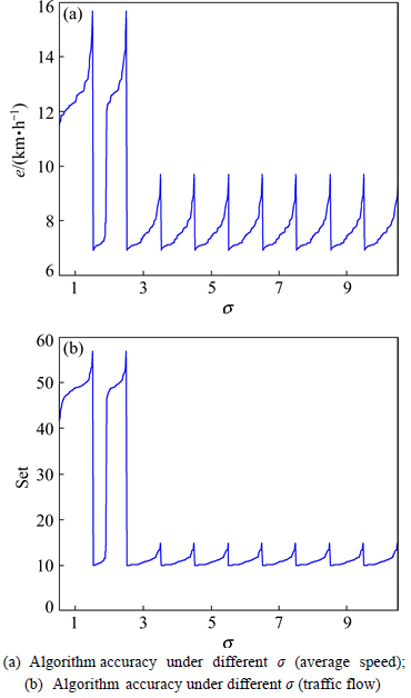
Fig. 3 Influence analysis of σ on algorithm:

From Fig. 4, we can see that the algorithm precision increases when the value of k increases; when the value of k increases from 9 to 10, the algorithm precision has little improvement.

3) Influence analysis of c on algorithm

Firstly, the experiment results when the value of c is 9 or 10 are retained. Then, the algorithm precisions under different c are counted and analyzed. The statistical results are shown in Fig. 5.

From Fig. 5, we can see that when the value of c Increases, the algorithm precisions basically increase; the optimal value of c is basically 5.

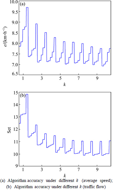
Fig. 4 Influence analysis of k on algorithm:

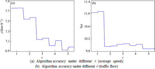
Fig. 5 Influence analysis of c on algorithm:

Based on the upper determination process of optimal parameters, the optimal parameters values for estimating average speed and traffic flow are basically the same, which can be obtained as listed in Table 4.

Table 4 Optimal parameters values

6.2 Experiment results

Based on the extraction of experimental data and the determination of algorithm parameters, the road traffic states of the target link could be estimated. The experiments focused on the estimation of speed and volume. To make the experiments results have more comparability, the road traffic states estimated based on simple historical data imputing and KNN were also obtained.

In addition, the estimation error indices, absolute error e, percentage error PE and the standard deviation of the absolute errors are computed. These indices are defined as

e=|S*-S|, ,        (16)

where S* is the road traffic state parameters estimated based on different means; v is the true road traffic state parameters; n is the number of samples.

Let e_ker and PE_ker denote absolute error and percentage error of the road traffic states estimated based on kernel-KNN matching of road traffic spatial characteristics, σ_ker denote the standard deviation of e_ker, e_KNN and PE_KNN denote absolute error and percentage error of the road traffic states estimated based on KNN matching of road traffic spatial characteristics, σ_KNN denote the standard deviation of e_KNN, e_sim and PE_sim denote absolute error and percentage error of the road traffic states estimated based on simple historical data imputing and σ_sim denote the standard deviation of e_sim.

6.2.1 Experiment results of estimated speed

The speed estimation results of the target link on June 19/25/26, 2011 are shown in Fig. 6.

The statistical results of the estimated speed based on different means are listed in Table 5.

6.2.2 Experiment results of estimated volume

The volume estimation results of the target link on June 19/25/26, 2011 are shown in Fig. 7.

The statistical results of the estimated speed based on different means on June 19/25/26, 2011 are listed in Table 6.

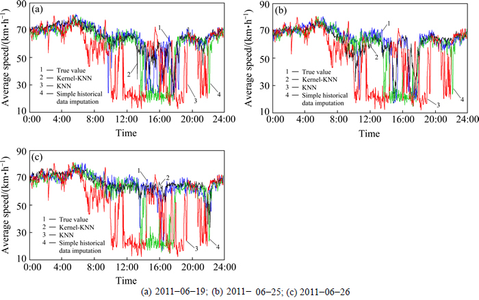
Fig. 6 Comparison of estimated results of speed through different means:

Table 5 Comparison of estimated results of speed

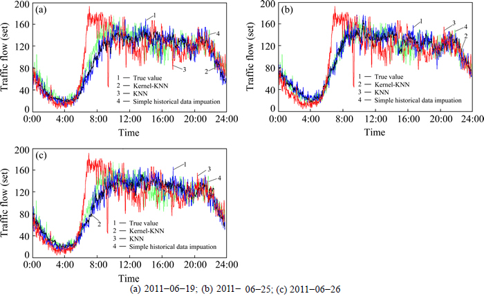
Fig. 7 Comparison of estimated results of volume through different means:

Table 6 Comparison of estimated results of volume

6.3 Statistical test

As the same theoretical background of the kernel-KNN and KNN, so it is necessary to assess the statistical significance of the estimations. We used a statistical test proposed by DIEBOLD and MARIANO. Based on Diebold and Mariano’s suggestion, the asymptotic test (S1) is employed in this study is applied, which is defined as

where d_i is the loss-differential series of kernel-KNN and KNN models, defined as

d_i=

and is the weighted sum of the available sample autocovariances:

where n is the sample size.

If the value of S₁ is not strikingly different with 0, the two models have the same ability for estimation. If the value of S₁ is strikingly positive, the loss-differential function of Kernel-KNN strikingly is greater than KNN, which means that the KNN model has better ability for estimation; if the value of S₁ is strikingly negative, the loss-differential function of kernel-KNN is strikingly smaller than KNN, which means that the kernel-KNN model has better ability for road traffic estimation.

The loss-differential series of the two models for the estimation of speed and volume are shown in Figs. 8 and 9.

The sample autocorrelation function (shown in Figs. 10 and 11), which decays quickly, indicates that the approximate stationarity is supported in the experiments.

The experiments results on different links are used for the statistical test. The statistical significance results are listed in Table 7.

From Table 7, we can find that kernel-KNN model has better ability for estimating speed and volume than KNN.

6.4 Analysis of experiment results

From the Tables 5, 6, and 7, Figs. 6 and 7, we can see the following.

1) Precision and stability of the results of speed and volume estimated based on kernel-KNN matching of road traffic spatial characteristics are both superior than other two algorithms.

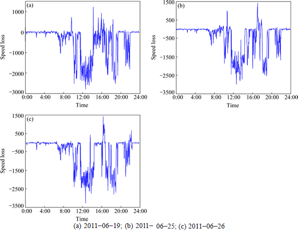
Fig. 8 Loss differential ((kernel-KNN)-KNN) of speed:

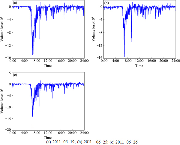
Fig. 9 Loss differential ((kernel-KNN)-KNN) of volume:

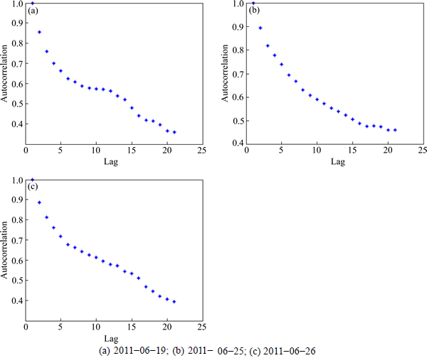
Fig. 10 Loss differential autocorrelations for speed estimation:

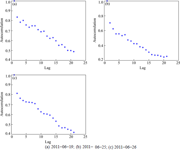
Fig. 11 Loss differential autocorrelations for volume estimation:

Table 7 Statistical significance results

From Tables 5 and 6, the following results can be obtained: ① Based on kernel-KNN matching of road traffic spatial characteristics, for the estimated speed and volume, the average absolute errors are 4.73 km/h and 8.68set respectively; the percentage errors are 7.41% and 8.74%, respectively; the standard deviation of the absolute error are 5.79 and 7.19, respectively. ② Based on KNN, for the estimated speed and volume, the average absolute errors are 15.94 km/h and 21.55 set respectively; the percentage errors are 24.94% and 21.72% respectively; the standard deviation of the absolute errors are 16.17 and 21.65, respectively.③ Based on simple historical data imputing, for the estimated speed and volume, the average absolute errors are 7.46 km/h and 13.84 set, respectively; the percentage errors are 11.64% and 13.96%, respectively; the standard deviation of the absolute error are 10.62 and 11.2 respectively.

From Table 7, we also can found that kernel-KNN model is strikingly superior to KNN.

2) Precision of the estimated results for speed is higher than volume.

The change regularity of volume is mainly determined by the regularity of people travel OD. But for different date, people travel OD changes more randomly. So, the change regularity of volume has certain random property. The change regularity of speed is not only affected by the regularity of people travel OD, but further affected by the running status of road infrastructure. So, the change of speed represents more regularity. The precision of speed is higher than volume when they are estimated based on the regularity of road traffic.

3) When the road traffic states change intensely, the precision of this road traffic states estimation algorithm decreases.

From the red circle signed in Fig. 8, we can see that: when the road traffic states changed sharply or frequent randomly, this algorithm adapted worse. This was mainly caused by two reasons: ① The RSRTRC cannot contain all road traffic states. ② The change of the target link’s road traffic states aren’t synchronized with the change of spatial correlated links. When the road traffic states changed sharply, it’s most likely that some incidents occurred, which was less in the RSRTRC in this experiment. To increase the performance of the algorithm, the RSRTRC should contain more road traffic state data, especially the data corresponding with incidents.

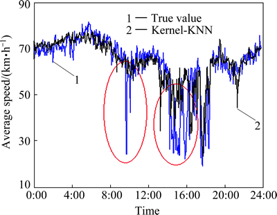
Fig.12 Example of estimated results of speed (2011-06-19)

4) This road traffic states estimation approach can be applied to all links with spatial correlation.

Though only freeways are selected in experiments to test and verify the algorithm, but from the description of the algorithm, it is easy to find that the road traffic states are estimated based on the spatial correlation between different links. The algorithm doesn’t have constraint for the types of links. So, the algorithm proposed in this paper has the generality property, it can also perform well with links of different types.

5) There are still some errors of the road traffic state estimated by this algorithm.

The errors are mainly caused by two reasons.① The first reason is that it is difficult to obtain the corresponding road traffic states with perfectly matching based on Kernel-KNN matching of road traffic spatial characteristics. This is mainly caused by the limitations of the RSRTRC. ② The second reason is that some deviations exist in the parameters. The process of determination of the optimal parameters is rough. For different road traffic state data sets, the optimal parameters determination is different. The selected optimal parameters are determined based on historical road traffic state data, so the current optimal parameters are different from the historical optimal parameters.

7 Conclusions

1) The multi-dimensional and multi-granularity road traffic state data sequences are mapped into high dimensions to construct the kernel function. Based on the Kernel-KNN matching of road traffic spatial characteristics matching, the road traffic states can be estimated. The kernel function of road traffic state data sequences can effectively improve the precision of the estimated road traffic states.

2) The experimental results prove that the traffic states calculated based on this algorithm is relatively accurate and stable. It could be applied to the analysis of regional traffic guidance and control.

3) During the next stage of research, we will study to improve the matching approach of the road traffic data sequences under sharply changed situations to improve the algorithm’s precision.

References

[1] XU Dong-wei. Multi-dimensional and multi-granularity acquisition of road traffic states [D]. Beijing: Beijing Jiaotong University, 2014. (in Chinese)

[2] ZHONG Ming, Sharma S, LIU Zhao-bin. Assessing robustness of imputation models based on data from different jurisdictions: Examples of Alberta and Saskatchewan, Canada [J]. Transportation Research Record: Journal of the Transportation Research Board, 2005, 1917(1): 116-126.

[3] YIN Wei-hao, Murray-Tuite P, Rakha H. Imputing erroneous data of single-station loop detectors for nonincident conditions: Comparison between temporal and spatial methods [J]. Journal of Intelligent Transportation Systems: Technology, Planning, and Operations, 2012, 16(3): 159-176.

[4] Haworth J, CHENG Tao. Non-parametric regression for space–time forecasting under missing data [J]. Computers, Environment and Urban Systems, 2012, 36(6): 538-550.

[5] RAY R D, Douglas B C. Experiments in reconstructing twentieth-century sea levels [J]. Progress in Oceanography, 2011, 91(4): 496-515.

[6] QU Li, LI Li, ZHANG Yi, HU Jian-ming. PPCA-based missing data imputation for traffic flow volume: a systematical approach [J]. IEEE Transactions on Intelligent Transportation Systems, 2009, 10(3): 512-522.

[7] schneider T. Analysis of incomplete climate data: estimation of mean values and covariance matrices and imputation of missing values [j]. journal of climate, 2001, 14(5): 853-871.

[8] LI Li, LI Yue-biao, LI Zhi-heng. Efficient missing data imputing for traffic flow by considering temporal and spatial dependence [J]. Transportation Research Part C: Emerging Technologies, 2013, 34: 108-120.

[9] Whitlock M E, Queen C M. Modelling a traffic network with missing data [J]. Journal of Forecasting, 2000: 19(7): 561-574.

[10] van Lint J W C, Hoogendoorn S P, van Zuylen H J. Accurate freeway travel time prediction with states-space neural networks under missing data [J]. Transportation Research Part C: Emerging Technologies, 2005, 13(5/6): 347-369.

[11] XU Dong-wei, DONH Hong-hui, JIA Li-min, TIAN Yin. A traffic state estimation method based on the road traffic information templates [C]// ICTIS 2013@ sImproving Multimodal Transportation Systems-Information, Safety, and Integration. ASCE, 2013: 934-940.

[12] XU Dong-wei, DONG Hong-hui, JIA Li-min, TIAN Yin. Road traffic states estimation algorithm based on matching of the regional traffic attracters [J]. Journal of Central South University, 2014, 21(5): 2100-2107.

[13] Roughan M, Zhang Yin, Willinger W, QIU Li-li. Spatio-temporal compressive sensing and internet traffic matrices (extended version) [J]. IEEE/ACM Transactions on Networking, 2012, 20(3): 662-676.

[14] XU Dong-wei, DONG Hong-hui, JIA Li-min, LI Hai-jian, FENG Yuan-jing. The estimation of road traffic states based on compressive sensing [J]. Transportmetrica B: Transport Dynamics, 2015, 3(2): 131-152.

[15] XU Dong-wei, DONG Hong-hui, JIA Li-min, QIN Yong. Virtual speed sensors based algorithm for expressway traffic states estimation [J]. Science China: Technological Sciences, 2012, 55(5): 1381-1390.

[16] XU Dong-wei, WANG Yong-dong, LI Hai-jian, QIN Yong, JIA Li-min. The measurement of road traffic states under high data loss rate [J]. Measurement, 2015, 69: 134-145.

[17] WU Tao. Kernels’ properties, tricks and its applications on obstacle detection [D]. Changsha: National University of Defense Technology, 2003. (in Chinese)

[18] LIN Mao-liu, Chen Chun-yu. A performance comparison of SVMs based on Fourier kernel and RBF kernel [J]. Journal of Chongqing University of Posts and Telecommunications, 2005, 17(6): 647-650.

(Edited by DENG Lü-xiang)

Foundation item: Projects(LQ16E080012, LY14F030012) supported by the Zhejiang Provincial Natural Science Foundation, China; Project(61573317) supported by the National Natural Science Foundation of China; Project(2015001) supported by the Open Fund for a Key-Key Discipline of Zhejiang University of Technology, China

Received date: 2015-06-23; Accepted date: 2015-12-10

Corresponding author: XU Dong-wei, PhD, Lecture; Tel: +86-571-88326202; E-mail:dongweixu@zjut.edu.cn