J. Cent. South Univ. Technol. (2008) 15(s1): 247-251

DOI: 10.1007/s11771-008-356-5

Autoregressive trispectrum and its slices analysis of magnetorheological damping device

CHEN Bing-san(陈丙三), HUANG Yi-jian(黄宜坚)

(College of Mechanical Engineering and Automation, Huaqiao University, Quanzhou 362021, China)

Abstract: A combined magnetorheological damper combined with rubber spring and magnetorheological damper is addressed. This type of damping device has inherited the merits of rubber spring and the magnetorheological damper. The test damping device is made up of combined magnetorheological damper, amplitude controller, signal collecting device, computer software for dynamic analysis, etc. When a zeromean and non-Gaussian white noise interfere with the device, a time series autoregressive(AR) model is conducted by using the sampled experimental data. Trispectrum and its slices analysis are emerging as a new powerful technique in signal processing, which is put forward for investigating the dynamic characteristics of the magnetorheological vibrant device. The present of trispectrum and its slices analysis change with the variation of controllable working magnetic field of the damper correspondingly. It is indicated that AR trispectrum and its slices analysis methods are feasible and effective for investigation of magnetorheological vibrant device.

Key words: magnetorheological fluids; combined magnetorheological damper; autoregressive (AR); trispectrum and its slices

1 Introduction

Magnetorheological (MR) fluid has significant characteristics fit for high technology and is a kind of smart soft matter being designed as a workable engineering material. The essential characteristic of MR fluids is their ability of reversible change from linear viscous liquids to semi-solid having controllable yield strength in milliseconds under a magnetic field. The other important properties of MR fluids are as follows: their mechanical simplicity, low power requirements, large force capacity, and robustness^[1]. Flow or shear properties of MR fluids are easily controlled to enable a variety of vibration control devices. A main application area for MR fluids is in dampers and mounts for use in semi-active or adaptive vibration control, which have attracted a great deal of attention in recent years. YANG^[2] developed a fundamental understanding of large-scale MR dampers for the purpose of designing and implementing these “smart” damping devices in large-scale structures. XIA^[3] presented an inverse model of the MR damper, i.e., the model can predict the required voltage so that the MR damper can produce the desired force to meet the requirement of vibration control of structures.

The interest in studying the dynamic characteristics lies in the fact that the higher order spectral characteristics of MR damping devices are important to control the vibrant devices. Higher order spectrum analysis is emerging as a new powerful technique in signal processing, which can describe nonlinear coupling, restrain Gaussian noise and reserve phase component. A number of studies of MR damping devices are pursued for modeling by using the spectral and other approaches, but few of these offer parametric trispectral analysis of vibrant mechanism.

The aim of this paper is the development of a fundamental understanding of the dynamic properties of the MR damping device with a new type of MR damper. By building the time series AR model, trispectrum and its slices analysis are used to asses the dynamic characteristics of the damping system and the damper. 

2 Work principle of MR damping device

The principle of MR damping device is shown in Fig.1. The device consists of an amplitude controller which adjusts the exciting force, the signal collecting device combined MR damper, computer software for dynamic analysis, etc. Combined MR dampers can achieve variable damping by changing the MR fluid flow resistance using a cylindrical gap under a variable magnetic filed. In addition, the rubber spring works alone without magnetic field.

A classical power law model of MR fluid should be used for accurate performance analysis and control of MR vibrant device:

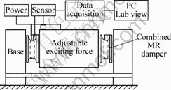
Fig.1 MR damping device

                                    (1)

where  T is the shear stress;  is the shear rate; η_a is the apparent viscosity, Pa?s, and can be represented by:

                         (2)

where  I is electric current, A; k(I) is consistency; index β(I) is a function of the electric current I.

The fluid resistance can be controlled by changing the electric currents, and the relationship between the fluid resistance f_d and applied electric current I can be expressed as:

            (3)

where  L is the length of the piston, m; R_po and R_ci are the radius of the piston and the inner radius of the cylinder, m; g is the gap between the piston and the cylinder, m; N is the turn number of the coil; u is the velocity of the piston, m/s.

Because of its complex structure, which makes it difficult to apply second moment analysis methods, the higher order cumulant analysis methods are developed for this system. By using trispectrum analysis we can obtain the useful dynamic information of the MR damping device.

3 Experimental equipments

The film sensors is used to detect temperature, displacement. The whole detecting, analyzing and controlling system based on NI virtual instruments are automatically operated by a computer.

 In experiments, the displacement and temperature signals from the high-speed data acquisition board PCI-MIO-16E-1 are used to control the applied electric current signal. Signals gathered are sent to dynamic signal analyzer NI-4552 for processing. The whole system is under the management of programs developed by the software platform LabVIEW. The A-D connector has 12 bits. The program is written by G language given by software LabVIEW and executed with a sampling frequency of 1000 Hz according to the desired control precision and the Nyguist sampling theorem.

4 AR trispectrum and its slices analysis

4.1 AR model

Detail information of the system contains abundant useful dynamic information generated by non-Gaussian zero-mean white noise a(t), shown in Fig.2. It is possible to set up AR model:

, (t=1, 2, …, N)        (4)

where  ψ_i(i=1, 2, …, p) donates AR coefficient; p donates the order of AR model. The high order cumulant of a(t) can be expressed with d_a,k:

              (5)

where  τ₁, τ₂,…, τ_k-1 are delays. Assume that τ₁=τ₂= τ_k-1=0，from Eqn.(5), we can obtain:

, , (6)

Then define  and  as Skewness and Kurtosis^[4], respectively. For symmetric distribution and yield unskewed output signal y(t), Skewness equals zero. For a Gaussian distribution, the Kurtosis is 3. Assume that delays are given as i₀=i₁-τ₁= i₂-τ₂=…= i_k-1-τ_k-1=i, then the high order cumulant of system output y(t) can be expressed as:

       (7)

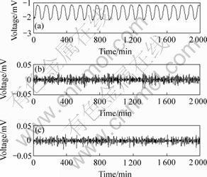
Fig.2 Colored a(t): (a) Sampled data y(t) at I=0 A; (b) Treated data by using wavelet a(t) at I=0 A; (c) Treated data by using wavelet a(t) at I=2 A

where  h(i) defines as the system’s unit pulse respond function.

4.2 High order spectrum

It is assumed that the cumulant sequences satisfy the bounding condition:

Under this assumption, the higher order spectra are usually defined in terms of the kth-order cumulants as their (k-1)-dimensional Fourier transforms, according to:

 (8)

where  f is frequency; H(f ) is the systemic transfer function; H^*(f ) is defined as the conjugate function of H(f ), S_y1,k(f₁, f₂, …, f_k-1) is defined as high order spectrum，also named high order cumulants spectrum, where k=1, 2, 3, …. The special spectra derived from Eqn.(8) are power spectrum P(f ) (k=2), bispectrum   B(f₁, f₂) (k=3) and trispectrum T(f₁, f₂, f₃) (k=4), respectively. Only power spectrum is real, the others are complex magnitudes. Here the emphasis is put on the analysis of trispectrum and its slices.

4.3 AR trispectrum

AR trispectrum can be defined as the three- dimensional Fourier transform of the cumulant function according to Eqn.(8):

                            (9)

In Eqn.(9), |f₁|≤π, |f₂|≤π, |f₃|≤π; H(f  ) is the transfer function of the system described in Eqn.(7), can be defined as:

                (10)

By using the parametric method of AR model to estimate model coefficient , which represents the coefficient of AR power spectrum, AR bispectrum, and AR trisepctrum. Combining Eqn.(10), substitute the coefficient in Eqn.(9) with γ, the amplitude of AR trispectrum can be obtained:

          (11)

The amplitude of the trispectrum is a function of three frequency variables and so requires four- dimensional space to display. Here it is attempted to display the magnitude of the entire trispectrum to give an overall picture of the trispectral information.

To achieve this, a sphere is drawn at each point in the trispectral space. The size and shade of the sphere represent the magnitude at that point: large dark spheres represent points of large magnitude, reducing across a grey scale to small light spheres which represent points of smallest magnitude. The spheres corresponding to small values are not drawn, to avoid the space being crowded by such spheres ^[4].

Magnitudes of the trispectrum for I=0, 1.0, 2.0 and 3.0 A are depicted in Fig.3. In Fig.3 dimension origin is located in the bottom hind corner of the graph and only the regions of positive angular frequencies (0-π) are displayed. The discrete trispectrum has 96 regions of symmetry and has been discussed detailedly^[5].

From Fig.3 it is clear to find that the energy distribution for I=0 is the biggest, and the largest magnitudes are at points (0, 0, 0), (π, 0, 0), (0, π, 0), (0, 0, π), (π, 0, π), (π, π, 0), (0, π, π), (π, 0, π), which are denoted by the large spheres. Also for I =1.0, 2.0, 3.0 A, the largest magnitude points exit and in the same positions. These points represent the largest vibration energy distribution of the damping device in different

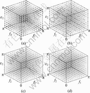
Fig.3 Trispectum TS^AR: (a) Trispectum for I=0; (b) Trispectum for I=1.0 A; (c) Trispectum for I=2.0 A; (d) Trispectum for I=3.0 A

states. The energy distribution decreases with the increase of the electric current, which explains that the absorption of the vibration energy increases with the enlargement of electric current. A better way to get the information is the slices analysis of the trispectrum. The method is described detailedly in the following.

4.4 2-D slices of trispectrum

When freezing one frequency of AR trisepctrum T^AR(f₁, f₂, f₃), taking f₃=C₁ (const) for example, the expression formula of AR trispectrum can be defined by:

                           (12)

It is more usual in high order spectrum literature to use Eqn.(12) as the definition of 2-D slices of AR trispectrum, the amplitude is:

      (13)

In traditional manner the 2-D slices of trispectrum are displayed in Fig.4. Fig.4 gives the slices TS^AR(f₁, f₂, 0). The amplitude of 2-D slices decreases with the increase

of the electric currents. The results are agreement with the conclusions gotten from Fig.3.

4.5 1-D slice of trispectrum

In order to extract more useful information of amplitude and frequency characteristics of signals intuitively, reflecting the dynamic characteristics of the damping device, another useful analysis method of 1-D slice spectrum is proposed here.

For f₂＝C₂ (const), combined with Eqn.(9) and Eqn.(12), the expression formula of 1-D slice of trispectrum is given as follows:

                           (14)

Therefore, the corresponding normalization amplitude of 1-D slice spectrum of trispectrum is defined as:

         (15)

1-D slice of trispectrum represents the relationship between amplitude and frequency, discribing the energy

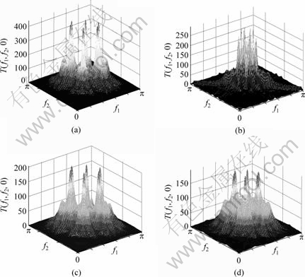
Fig.4 2-slices of trispectrum: (a) TS^AR(f₁, f₂, 0) of I=0 A; (b) TS^AR(f₁, f₂, 0) of I=1.0 A; (c) TS^AR(f₁, f₂, 0) of I=2.0 A; (d) TS^AR(f₁, f₂, 0) of I=3.0 A

distribution in the frequency domain. From Fig.5, it can be easily obtained that the reduction of system energy with the increasement of the electric currents, which is consistent with the analysis of Fig.3 and Fig.4.

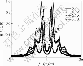
Fig.5 1-D slice of trispectrum

5 Conclusions

Estimating and analyzing the dynamic characteristics are important to design and control the magnetorheological damping system. Experiments and the time series analysis demonstrate that.

1) When a zeromean and non-Gaussian white noise interferes with the magnetorheological damping device, AR model of fourth-order cumulant can be established for investigating the dynamic characteristics of MR system.

2) The trispectrum gives an indication of the correlation between the phases of different frequency components f₁, f₂, f₃.

3) Since time series model is a parametric model, the trispectrum and its slices are smooth.

References

[1] YING Z G, Ni Y Q, Ko J M. Semi-active optimal control of linearized systems with multi-degree of freedom and application[J]. Journal of Journal of Sound and Vibration, 2005, 279(1/2): 373-388.

[2] YANG G Q. Large-scale magnetorheokogical fluid damper for vibration mitigation: Modeling, testing and control[M]. Indiana: University of Notre Dame, 2001.

[3] XIA Pin-qi. An inverse model of MR damper using optimal neural network and system identification[J]. Journal of Sound and Vibration, 2003, 266(5): 1009-1023.

[4] COLLIS W B, WHITE P R, HAMMOND J K. Higher-order spectra: The bispectrum and trispectrum[J]. Mechanical System and Signal Processing, 1998, 12(3): 375-395.

[5] ZHANG Xian-da. Time series analysis[M]. Beijing: Tsinghua Univ Press, 1999: 11-13. (in Chinese)

(Edited by CHEN Ai-hua)

Foundation item: Project(2005H035) supported by Fujian Province of China

Received date: 2008-06-25; Accepted date: 2008-08-05

Corresponding author: CHEN Bing-san, PhD; Tel: +86-595-22689843; E-mail: bschen126@163.com