J. Cent. South Univ. Technol. (2011) 18: 2074-2079

DOI: 10.1007/s11771-011-0945-6

RS-SVM forecasting model and power supply-demand forecast

YANG Shu-xia(杨淑霞), CAO Yuan(曹原), LIU Da(刘达), HUANG Chen-feng(黄陈锋)

School of Economics and Management, North China Electric Power University, Beijing 102206, China

? Central South University Press and Springer-Verlag Berlin Heidelberg 2011

Abstract: A support vector machine (SVM) forecasting model based on rough set (RS) data preprocess was proposed by combining the rough set attribute reduction and the support vector machine regression algorithm, because there are strong complementarities between two models. Firstly, the rough set was used to reduce the condition attributes, then to eliminate the attributes that were redundant for the forecast, Secondly, it adopted the minimum condition attributes obtained by reduction and the corresponding original data to re-form a new training sample, which only kept the important attributes affecting the forecast accuracy. Finally, it studied and trained the SVM with the training samples after reduction, inputted the test samples re-formed by the minimum condition attributes and the corresponding original data, and then got the mapping relationship model between condition attributes and forecast variables after testing it. This model was used to forecast the power supply and demand. The results show that the average absolute error rate of power consumption of the whole society and yearly maximum load are 14.21% and 13.23%, respectively, which indicates that the RS-SVM forecast model has a higher degree of accuracy.

Key words: rough set (RS); support vector machine (SVM); power supply and demand; forecast

1 Introduction

The traditional time series forecast methods mostly use causal sequence regression model and the time series model. The established model cannot reflect the intrinsic structure and the complex characteristics of the dynamic data comprehensively, scientifically or constitutionally, which causes the loss of the information [1]. As a new algorithm based on the principle of minimized structural risk, support vector machine (SVM) has incomparable advantages to other algorithms based on the minimized experience risk principle [2].

However, it cannot simplify the dimensions when using SVM to process the information, and this will lead to a longer time of SVM training when the space dimension of input information is greater [3-4]. However, RS method can take out the redundant information of the data by discovering the relationship among the data, and simplify the dimensions of information input space. RS theory has weaker error tolerance and generalization abilities, while SVM method has a good ability of curbing noise and generalization [5]. Therefore, if using RS method to eliminate redundant information, training samples can be simplified and SVM input data can be reduced, which will shorten the training time [6].

2 Thought of rough set reduction

2.1 Standardization of raw data

The number of indexes which is used to predict the power supply and demand is large, and index measurement units are different. Moreover, date values have relatively large differences. If these raw data are not standardized but take attributes reduction by rough set algorithm, bad result will appear. Therefore, the minimum-maximum standardization method should be used to standardize raw data before taking reduction algorithm. Assume attribute (including condition attribute and forecast attribute)  and A=  A is finite nonempty set, C={c₁, c₂, …, c_m} is condition attribute, and D={d₁, d₂, …, d_n} is forecast attribute, where r_i is its attribute value. If max{r_i} and min{r_i}, i=1, …, n are the maximum value and minimum value of attribute r, respectively, two formulas can be used to map r into [0, 1] interval:

                                                  (1)

                                   (2)

Equation (1) is suitable for attribute index which positively correlates with forecast attribute, and Eq.(2) is suitable for attribute index which negatively correlates with forecast attribute.

2.2 Continuous attribute discretization

Traditional rough set theory can only process discrete data, but some index data during prediction are continuous. Continuous index data can be discrete by using equal division method.

Equal division method can be divided into two groups. One group is equal width interval method, which divides continuous value interval into N intervals (N is a given discrete number). Assume that the raw interval is [a, b], and N equal width intervals are [a, a+(b-a)/N], [a+(b-a)/N, a+2(b-a)/N], …, [b-(b-a)/N, b]. The other group is equifrequency interval method, which divides raw interval into N intervals (N is a given discrete number), getting approximately equal object number in every small interval. Namely, take the same number of attribute value samples starting with a_min as an interval every time. If the total number of the attribute value is M and the number of discrete interval is N, then the sample number in every interval is M/N.

2.3 Rough set reduction

During the forecasting process, each reduced set can take place of the whole condition attribute set without altering the original dependent relationship. Therefore, the best reduced set should be determined [7-10]. In attributes reduction, it is assumed that attribute  is a reduction of C. Only if POS_B(D)=POS_C(D), then each attribute of B is indispensable for D. Attribute reduction is marked as red(B, D). Its steps are: finding out the core of attribute reduction set, then using reduction algorithm to calculate the reduction set, and determining the best one with a certain evaluation criterion.

According to the forecast information table, condition attribute C={c₁, c₂, …, c_m}, forecast attribute D={d₁, d₂, …, d_n} and corresponding value V, the importance of condition attributes for the forecast attribute is calculated, which can be determined by calculating the dependence degree of the forecast attribute D and condition attribute [11].

Suppose that condition attribute is c_i, i=1, 2, …, m; forecast attribute is d_j, j=1, 2, …, n. Then, the dependence degree of forecast attribute d_j to condition attribute c_i is presented as

0≤γ(c_i, d_j)≤1                   (3)

where  is the positive region of c_i to d_j, and card(*) is the base of the calculation region.

Assuming  then the importance degree of  to d_j is presented as

                           (4)

This algorithm firstly calculates the importance of each condition attribute to the forecast attribute, then adds the condition attributes into the attributes set redU followed by their importance degree from high to low. Review the dependence degree between the attribute set redU and forecast attribute, and the important condition attributes will be included in redU. Then, the attributes are removed from the attribute set redU one by one from ones with higher importance degree to lower. If removed attribute causes the changes of dependence degree, then resume it. The last remaining attribute set is the best reduced set, namely the most important condition attribute.

3 Forecasting process of RS-SVM

3.1 Support vector machine regression algorithm

The basic thought of support vector machine regression algorithm is mapping data x in input space to a N-dimensional feature space by using a nonlinear mapping f, making a linear mapping in the N- dimensional space, and realizing the regression estimation through linear minimization.

The predicting thought of the regression model support vector machine is as follows [12-14]: Given a

data point  where x_i is the input vector,

d_i is the expected value, and n is the total number of the data. Support vector machine adopts Eq.(5) to estimate the function:

                                                   (5)

where f(x) is the nonlinear mapping from input space to N-dimensional feature space. The coefficients ω and b are estimated by minimizing Eq.(6):

                (6)

                                (7)

In the regularization risk functional given in Eq.(7),

the first part  which is measured by

insensitive loss function, is the empirical risk. Loss function is used in expressing the decision-making function which is given by Eq.(5) with the sparse data. c is a positive constant, and it decides the balance between the empirical risk and the regularization part. The second

part  is the regularization part.

To obtain the coefficients ω and b, it needs to introduce the relaxation variables  and  and minimize Eq.(8):

                        (8)

s.t.                         (9)

After the introduction of Lagrange’s multipliers  and  the decision-making function (3) changes to

                       (10)

s.t.  i=1, …, n

where  and  are Lagrange’s multipliers, K(x, x_i) is called the kernel function. For minimizing Eq.(8) under the constraint conditions Eq.(9), it can simplify the convex optimization problem to be a quadratic optimization problem which seeks for vector ω after the introduction of the Lagrange’s multipliers. In such a case, it must obtain the maximum quadratic model before

finding out the desired coefficient

                      (11)

The constraint condition of the parameters  and  in Eq.(11) is

  i=1, …, n

By controlling two parameters c and ε in the quadratic optimization method, it can control (even if in the N-dimensional space) the generalization of the support vector machine. According to conditions K-T in the convex quadratic programming, only parts of these coefficients  in Eq.(11) possess nonzero values and their corresponding data points are just the support vectors. These data locate on or outside the boundary. The coefficients  of other data points in Eq.(11) are all equal to zero, so it is confirmed that only the support vectors among all the data can solve the decision-making function. Generally speaking, the larger the ε value is, the less the number of the support vectors is and the sparser the solution expression is. However, large ε value can also reduce the approximating precision of the data, so ε is also the balance factor between the density of the data points and the sparse degree of the solution expression.

To calculate the parameter b, the K-T condition mentioned above which was used in solving the convex quadratic programming problems may be adopted. The main thought is to select the Lagrange’s multipliers  and  which can determine the forecast error d_k=f(x_k)- y_k uniquely. Under the condition of the Vapnik’s ε insensitive loss function (namely |y_i-f(x_i)|ε=max{0, |y_i-f(x_i)|-ε}), the process of selecting Lagrange’s multipliers means to select data x_k on the boundary to obtain corresponding value of  and  as the exact value of the forecast value  has been known. Considering the stability, it can adopt the average value  of all points x_k on the boundary to obtain b, namely

                   (12)

In Eq.(11), K(x_i, x_j) is called the kernel function, the value of which equals the inner product of two vectors x_i and x_j in their feature space φ(x_i) and φ(x_j), namely and all functions that satisfy Mercer condition can be taken as kernel function.

The forms of the kernel function as well as its parameter determination decide the type and the complex degree of the learning machine. At present, the most commonly used kernel functions mainly include the following three kinds:

1) Polynomial kernel function:

d=1, 2, …                               (13)

2) Gauss kernel function (RBF kernel function):

                                         (14)

3) Sigmoid kernel function:

                            (15)

Support vector machine of regression model avoids the problems of over-study and owe-study by minimizing

the training error  and  (simplify

the complexity of the learning method, thus reducing the confidence interval of the error). In the traditional least squares regression method, ε usually is zero; moreover, the data are not mapped to the N-dimensional space for handling. Support vector machine regression algorithm is a more practical and flexible method to solve the regression problems.

3.2 RS-SVM forecasting model

RS-SVM forecasting processes are shown in Fig.1.

3.3 Calculation process of SVM algorithm based on matlab6.5

According to Refs.[15-16], after adopting kernel function, the program with matlab6.5 is designed to realize the above calculation process. Input historical data of condition attribute and forecast attribute. By controlling parameters c, ε and kernel parameter, generalization abilities and fitting degree of SVM can be controlled. c is used to compromise between model complexity and approximation error. The larger c value is, the better fitting degree of data is. ε is used to control the number of support vector. As ε value is big, support vector is less and fitting degree is low. The adopting of kernel parameter also has some effects on fitting degree. In a word, the adoption of the three parameters determines fitting degree. After determining parameters  c, ε and kernel parameter, input training sample (data of condition attribute and forecast attribute), coefficients ω and b, then the number of support vector and corresponding value  can be worked out. Next by inputting the test samples, fitting result can be got.

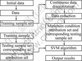
Fig.1 Forecasting model table based on RS-SVM

4 Power supply-demand forecast based on RS-SVM forecasting model

4.1 Forecasting information table of power supply and demand establishing

Establish the power supply-demand forecasting information table T=(U, A, V, f), where U is the domain,  C={c₁, c₂, …, c_m} is the condition attribute, including GDP, the primary industry output value, the second industry output value, the tertiary industry output value, energy efficiency improvements, industrial structure changes, population, disposable income of urban residents, disposable income of rural residents, power price (fuel price index) and other indicators. D= {d₁, d₂, …, d_n}, is the forecast attribute, including the whole society power consumption and yearly maximum

load.  where V_α is the range of attribute α, f

is an information function designating attribute value of each object in U. Relative data from 1985-2004 was chosen (Omit. data sources: China Electric Power Yearbook, China Statistical Yearbook).

4.2 Power supply-demand forecasting indexes handling

Make the data standardization (with results abbreviated), then adopt the equal-width interval method to disperse the condition attribute set {GDP, the primary industry output value, the second industry output value, the tertiary industry output value, energy efficiency improvements, industrial structure changes, population, disposable income of urban residents, disposable income of rural residents, power price}. Adopt the equal- frequency interval method to disperse the forecast attribute set {whole society power consumption, yearly maximum load}, then code the discrete values of the attributes with 0, 1, 2, …, and the discrete results of the condition attribute data can be obtained (with results abbreviated).

Make attribute reduction with the condition attribute set and the forecast attribute set, respectively, then get the optimum reduction attribute set of whole society power consumption {GDP, the primary industry output value, the second industry output value, the tertiary industry output value, energy efficiency improvements, industrial structure changes, population, disposable income of urban residents} and the optimum reduction attribute set of the yearly maximum load {GDP, the primary industry output value, the second industry output value, the tertiary industry output value, energy efficiency improvements, industrial structure changes, population, disposable income of urban residents}.

Use the two optimum reduction attribute set obtained above, respectively, to establish the power supply-demand forecasting models based on SVM regression algorithm. Adopt Gauss kernel function K(x,y)=

 and design the program with matlab6.5.

4.3 Power supply-demand forecast

Input the history data of whole society power consumption, GDP, the second industry output value, the tertiary industry output value, energy efficiency improvements, industrial structure changes, disposable income of urban residents from 1985-2000 as the training samples.

According to Refs.[17-18], c=90, σ²=35 and ε=0.05 were chosen. Then, it was known that ω=228.176, b= 46.13 and support vector number n=10 through program operation.

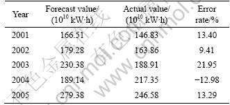
Input the testing samples, then the forecast results of the whole society power consumption from 2001 to 2005 are listed in Table 1.

Input the history data of the yearly maximum load, GDP, the second industry output value, energy efficiency improvements, industrial structure changes, disposable income of urban residents from 1985 to 2000 as the training samples into the program.

Table 1 Forecasting results of whole society power consumption

According to Refs.[17-18], c=100, σ²=28 and ε=0.12 were chosen. Then, it was known that ω=317.265, b=59.78, and support vector number n=12 through program operation.

Input the testing samples, then the forecast results of yearly maximum load from 2001 to 2005 are listed in Table 2. The comparisons between actual value and forecast value are shown in Figs.2-4.

Table 2 Forecasting results of yearly maximum load

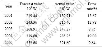
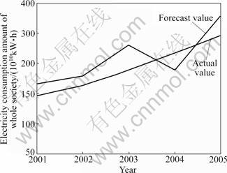
Fig.2 Actual value and forecast value of whole society power consumption from 2001 to 2005

It can be seen from the above calculated results that the average absolute error rate of whole society power consumption is 14.21%, and the average absolute error rate of yearly maximum load is 13.23%.

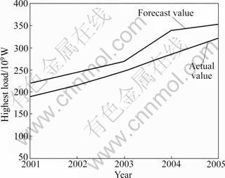
Fig.3 Actual value and forecast value of yearly maximum load from 2001 to 2005

Fig.4 Error rate curves

5 Conclusions

1) RS-SVM forecasting model can take out the redundant information of data by discovering the relationship among the data, and simplify the dimensions of information input space.

2) It also has a good ability of curbing noise and generalization, which will shorten the training time and improve the forecast accuracy. Therefore, RS-SVM forecasting model is especially suitable for forecasting with larger input space dimensions.

3) The forecasting accuracy is just related with c, ε and the selected kernel function by using this method. As long as the parameters have been chosen properly, the forecast can achieve satisfactory results.

References

[1] LI Yan-bin, LI Cun-bin, SONG Xiao-hua. Prediction model of improved artificial neural network and its application [J]. Journal of Central South University: Science and Technology, 2008, 39(5): 1054-1058. (in Chinese)

[2] MOSTAFA S, SADOGHI Y H, MAHMOUD N. Relaxed constraints support vector machines for noisy data [J]. Neural Computing and Applications, 2011, 20(5): 671-685.

[3] TIAN Jiang, GU Hong, LIU Wen-qi. Imbalanced classification using support vector machine ensemble [J]. Neural Computing and Applications, 2011, 20(2): 203-209.

[4] ANGUITA D, GHIO A, PISCHIUTTA S. A support vector machine with integer parameters [J]. Neurocomputing, 2008, 72(1/2/3): 480- 489.

[5] JIANG Shao-hua, GUI Wei-hua, YANG Chun-hua, DAI Xian-jiang. Fault diagnosis method based on rough set and least squares support vector machine and its application [J]. Journal of Central South University: Science and Technology, 2009, 40(2): 447-451. (in Chinese)

[6] THANGAVEL K, PETHALAKSHMI A. Dimensionality reduction based on rough set theory: A review [J]. Applied Soft Computing, 2009, 9(1): 1-12.

[7] XIE Gang, ZHANG Jin-long, LAI K. Variable precision rough set for group decision-making: An application [J]. International Journal of Approximate Reasoning, 2008, 49(2): 331-343.

[8] MASAHIRO I, YUKIHIRO Y, YOSHIFUMI K. Variable-precision dominance-based rough set approach and attribute reduction [J]. International Journal of Approximate Reasoning, 2009, 50(8): 1199-1214.

[9] QIAN Yu-hua, LIANG Ji-ye, WITOLD P. Positive approximation: An accelerator for attribute reduction in rough set theory [J]. Artificial Intelligence, 2010, 174(9/10): 597-618.

[10] HEDAR A, WANG J, FUKUSHIMA M. Tabu search for attribute reduction in rough set theory [J]. Soft Computing, 2008, 12(9): 909-918.

[11] LI Liang-min, WEN Guang-rui, WANG Sheng-chang. Parameters selection of support vector regression based on genetic algorithm [J]. Computer Engineering and Applications, 2008, 44(7): 23-26. (in Chinese)

[12] JERZY M. The forecasting model based on wavelet support vector machine and multi-elitist PSO [J]. Advances in Intelligent and Soft Computing, 2011, 103: 335-342.

[13] WU Qi, LAW R. An intelligent forecasting model based on robust wavelet v-support vector machine [J]. Expert Systems with Applications, 2011, 38(5): 4851-4859.

[14] NIU Dong-xiao, WANG Yong-li, MA Xiao-yong. Optimization of support vector machine power load forecasting model based on data mining and Lyapunov exponents [J]. Journal of Central South University of Technology, 2010, 17(2): 406-412.

[15] CHEN Qi-mai, CHEN Sen-ping. Sample selection algorithm based on kernel function in support vector machine [J]. Computer Engineering and Design, 2010, 31(10): 2266-2269.

[16] JIANG Shao-hua, GUI Wei-hua, YANG Chun-hua, TANG Zhao-hui. Method based on kernel principal component analysis and support vector machine and its application [J]. Journal of Central South University: Science and Technology, 2009, 40(5): 1323-1328. (in Chinese)

[17] CHEN Ran, SUN Dong-ye, QIN Da-tong, HU Feng-bin. A novel engine identification model based on support vector machine and analysis of precision-influencing factors [J]. Journal of Central South University: Science and Technology, 2010, 41(4): 1391-1397. (in Chinese)

[18] HUANG Chen-feng. Research on power supply-demand early warning based on rough set and support vector machine [D]. Beijing: North China Electric Power University, 2005. (in Chinese)

(Edited by YANG Bing)

Foundation item: Project(70901025) supported by the National Natural Science Foundation of China

Received date: 2011-04-24; Accepted date: 2011-09-23

Corresponding author: YANG Shu-xia, Professor, PhD; Tel: +86-10-51963881; E-mail: bjysx216@126.com