J. Cent. South Univ. (2016) 23: 2230-2241

DOI: 10.1007/s11771-016-3281-z

Remaining useful life estimation based on Wiener degradation processes with random failure threshold

TANG Sheng-jin(唐圣金), YU Chuan-qiang(于传强), FENG Yong-bao(冯永保),

XIE Jian(谢建), GAO Qin-he(高钦和), SI Xiao-sheng(司小胜)

High-Tech Institute of Xi’an, Xi’an 710025, China

Central South University Press and Springer-Verlag Berlin Heidelberg 2016

Abstract: Remaining useful life (RUL) estimation based on condition monitoring data is central to condition based maintenance (CBM). In the current methods about the Wiener process based RUL estimation, the randomness of the failure threshold has not been studied thoroughly. In this work, by using the truncated normal distribution to model random failure threshold (RFT), an analytical and closed-form RUL distribution based on the current observed data was derived considering the posterior distribution of the drift parameter. Then, the Bayesian method was used to update the prior estimation of failure threshold. To solve the uncertainty of the censored in situ data of failure threshold, the expectation maximization (EM) algorithm is used to calculate the posteriori estimation of failure threshold. Numerical examples show that considering the randomness of the failure threshold and updating the prior information of RFT could improve the accuracy of real time RUL estimation.

Key words: condition based maintenance; remaining useful life; wiener process; random failure threshold; bayesian; EM algorithm

1 Introduction

Remaining useful life (RUL) estimation is central to condition based maintenance (CBM), and it plays an important role in maintenance strategy selection, inspection optimization, spare parts provision, and life extension [1-4]. The RUL of an asset is formally defined as the length of time from present time to the end of useful life. Traditional failure time analysis methods for RUL estimation are heavily dependent on time-to-failure data, or lifetime data. However, some critical assets are so valuable that it is expensive to obtain enough failure information. Moreover, for the long life assets, it is hard to obtain enough failure data in a short time even through the accelerated life test. Therefore, the failure data are scarce in reality. In such cases, the degradation modeling based on the available condition monitoring (CM) information can be used for RUL estimation from an economical and practical viewpoint [4-7].

For the RUL estimation based on the CM data, the degradation trend should be modeled through the physics of failure models or stochastic models. However, it is difficult to obtain the underlying physical failure mechanisms of complex systems in advance. In contrast, the stochastic models fit the degradation paths directly through the CM data without relying on any physical failure mechanism. And, some nice mathematical properties of stochastic models can be used to analyze the estimated RUL. Wiener degradation process is a type of statistics-based data driven methods, which has a drift term and a noise term modeled by Brownian motion. Since the Wiener process can provide a good description of system’s dynamic characteristic due to its non-monotonic property, it has been widely used to model degradation processes, such as, gyros [8], laser generators [9], bridge beams [10], LEDs [11], continuous stirred tank reactors [12], hard disk drives [13], lithium-ion batteries [14-15], micro-electro-mechanical systems (MEMSs) [16], and rotating element bearings [17-18]. The RUL estimation methods based on the Wiener degradation process have gained much attention in recent years [19-20].

In general, there are two main factors that determine the RUL, which are the degradation paths and the failure threshold. The current research focus is to study the influence of degradation paths to RUL estimation and to find the probability density functions (PDF) or cumulative probability functions (CDF) of the RUL or lifetime of the Wiener process by assuming a fixed and known threshold. The PDFs of RUL for different forms of Wiener process based degradation paths have been studied in recently years, such as Wiener processes with random effects [9-10], nonlinear degradation process [8, 21-23], and latent degradation [14, 24-26]. To incorporate the real time degradation information into the estimated RUL, the modeling parameters are updated to make the estimation adapt to the item’s individual characteristic. Thus, the current observed CM data and the uncertainties of the estimated parameters are considered for estimating the PDFs of the RUL [4]. The threshold in the above research is chosen as a fixed and known value based on the engineering experience, the past failure data, or the accepted industrial standards.

However, the failure threshold of many degradation paths is not known and fixed due to the following reasons: 1) the failure threshold can vary appreciably among users of products; 2) the level of degradation that will cause a failure is not explicitly known [27]; and 3) there is uncertainty of the threshold determined by the engineering experience or the past failure data. Therefore, random failure threshold (RFT) exists widely in practice, such as vibration level of bearings [28], the milling machine [29], and fatigue degradation [30]. The influence of RFT to the RUL estimation has already been studied in the random effect regression model, proportional hazard model, and Gamma process [31-33]. USYNIN et al [31] provided an integral expression of the PDF of the RUL for the Wiener process. However, the distribution of the RFT and the analytical form of the RUL with RFT are not given. WANG et al [12] used the exponential distribution with a scale parameter and a location parameter to represent the RFT and give the integral expression of the probability density function. However, the analytical form of the RUL with RFT is also not given. WEI et al [29] used the traditional normal distribution to model RFT and derive the analytical form of the RUL. However, the limit of RFT to be positive is not considered in the RFT modeling.

In general, it is hard to obtain enough data of failure threshold since some products own high reliability and long life or the tests to obtain failure information are very expensive. Therefore, the prior estimation of failure threshold is often not very accurate. If the estimated failure threshold is larger than the real failure threshold, it would delay the maintenance time, cause failure maintenance, and decrease the system reliability and maintenance costs. Conversely, if the estimated failure threshold is smaller than the real failure threshold, it would cause premature maintenance and decrease the maintenance costs. As a result, the prior estimation of failure threshold should be updated when the products have been used after a period of time. However, due to application of CBM techniques, most products are no longer used when the products approach to the end of life. Therefore, the in situ data of failure threshold are censored, and the real failure thresholds are unknown. However, it is difficult to obtain the estimation of failure thresholds by the traditional maximum likelihood estimation (MLE) method.

From the above analysis, it is clear that the RUL estimation with RFT has not been studied thoroughly. To solve this problem, the following issues need to be addressed: 1) to describe the distribution of the RFT; 2) to obtain the analytical PDF and mean of RUL with the RFT; and 3) to update the prior estimation of failure threshold with a simple method.

In this work, the above issues are addressed via the Wiener based degradation process with the RFT. Firstly, a truncated normal distribution (TND) is proposed to describe the RFT. Secondly, the analytical form of the PDF and the mean of lifetime are proposed in the sense of the first hitting time (FHT), and the analytical PDF and mean of the RUL when the current CM data are applied are proposed for the real time RUL estimation. This is the main contribution of the paper since the uncertainties in both the estimated parameter and the RFT are incorporated simultaneously. Then, we use the Bayesian method to update the prior estimation of failure threshold. To solve the uncertainty of the censored in situ data of failure threshold, we use the expectation maximization (EM) algorithm to calculate the posteriori estimation of failure threshold. This is another contribution of this work, which is not fully explored before. Finally, a numerical example is presented to illustrate the application and usefulness of the proposed method.

2 Modeling random failure threshold

2.1 Problem description

As discussed previously, new developments are needed to model the Wiener degradation process with the RFT. Unlike the fixed threshold, the RFT is commonly represented by a failure zone, i.e. the item only fails according to a failure zone rather than a specific fixed threshold [12]. Therefore, how to model the RFT is the foremost problem to be settled. In general, the failure threshold in the failure zone should be greater than the initial value of the degradation process. For example, let X(t) represent the degradation process and set X(t)=0 without loss of generality; it is known that the failure threshold (w) follows that w>0. Thus, the first limit of the selection of the probability distribution for RFT is that the domain should be [0, +∞). Then, only exponential distribution, gamma distribution, inverse Gaussian distribution, etc., representing the nonnegative random variables, can be used to model the RFT.

Figure 1 illustrates the modeling principle of degradation process with the RFT. The RFT is characterized by a random variable with PDF, f(w), and the degradation process is described by a Wiener processwith random drift parameter. To derive the PDF of the RUL, the distribution of the RFT should be considered. When the CM information reaches X(t) at time t, the drift parameter is updated via the current CM data. However, the error may be produced by using the original probability function of the RFT, like inverse Gaussian distribution, gamma distribution, etc. The reason is that for a specific item, the failure threshold should be greater than X(t) on the condition that the item does not fail at time t. In other words, the distribution of the RFT changes when the CM data are newly observed for the real time RUL estimation. This produces another limit of the selection of the probability distribution for RFT. The existing papers do not consider these two limits [29] or only consider the first limit of the RFT [12], the second limit is first considered in this work. In the next subsection, the truncated probability function is used to solve this problem.

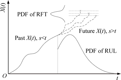
Fig. 1 Illustration of RFT modeling principle

2.2 Truncated normal distribution

Essentially, the distribution of the RFT for real time RUL estimation is a truncated probability distribution. In this work, the truncated normal distribution (TND) is used to represent the RFT. If Z~N (μ, σ²) and Z are truncated by Z>0, then this type of TND can be written as Z~TN (μ, σ²). Suppose that w~TN (μ_w, , the PDF and mean of w can be written as [34]

     (1)

     (2)

If μ_w~σ_w, then we have Φ(μ_w/σ_w)≈1 and Thus, the TND approximately turns into traditional normal distribution. Note that the TND is based on the traditional normal distribution. This methodology could be extended to other truncated probability distribution. The key issue of RUL estimation with the RFT is to derive the PDF of the RUL with RFT, which is addressed in the following section.

3 Degradation modeling and RUL estimation with RFT

3.1 Degradation model

In this section, the conventional Wiener process with linear drift is applied to model the degradation process for RUL the estimation with RFT. Let X(t) denote the degradation value at time t, the degradation process can be represented as follows

                     (3)

where λ is the drift parameter, and B(t) is the standard Brownian motion which represents the stochastic dynamics of the degradation process. Without loss of generality, X(0) is assumed to be zero. As the progression of the degradation is governed by the drift parameter λ, it is assumed that λ is a random parameter to represent the heterogeneity among different items, and σ_B is fixed which is common to all items. Moreover, λ is assumed to be s-independent with B(t).

3.2 Lifetime distribution with RFT

The main focus of the RUL prediction is to derive the analytical distribution of RUL. In this section, the RUL distribution is obtained under the concept of the first hitting time (FHT) of the degradation process. First, the definition of the failure time T can be represented as follows.

                  (4)

where w denotes the RFT. In this work, it is assumed that w obeys the TND.

In the sense of the FHT, it is well-known that the Wiener process crossing a constant threshold obeys an inverse Gaussian distribution [35]. Accordingly, given that w is a fixed value, the PDF, mean and variance can be obtained as follows.

           (5)

                  (6)

In general, the drift parameter can be represented as a random parameter to represent the heterogeneity among different items, which is called random effects. In this work, it is assumed that If the random effects are considered, the PDF and mean of FHT can be formulated as follows [9].

     (7)

                       (8)

For the lifetime estimation, it commonly follows that. As discussed previously, the TND can be approximated as the traditional normal distribution. Therefore, we use the traditional normal distribution to model RFT for the lifetime estimation. To derive the PDF of the lifetime with the RFT, the following lemma is first presented.

Lemma 1: If and B∈R, C∈R⁺, then

    (9)

The proof of Lemma 1 involves complicated mathematical transformation. For more details of the proof, see the proof of Theorem 3 in Ref. [8] and the proof of Theorem 4 in Ref. [36].

Based on Lemma 1, the PDF of the lifetime with the RFT can be obtained by the law of total probability in the following theorem.

Theorem 1: For the degradation process X(t) given in Eq. (3), if the PDF and mean of the RUL can be written as

    (10)

          (11)

where D(·) is the Dawson function.

The proof is omitted here since the steps are routine. In particular, if the in Eqs. (10) and (11) are set to be zero, the PDF and mean of the RUL with RFT can reduce to the case with a fixed value. In the following, we consider updating the drift parameter based on the CM data for RUL estimation.

3.3 RUL estimation with RFT

It is noted that the estimation by the historical data or the accelerated degradation test reflects the population degradation information. To make the estimation adapt to the item’s individual characteristic and reduce the uncertainty of the estimation, the drift parameter is updated for real time RUL estimation [36-38]. There are many methods for updating the drift parameter in the framework of Bayesian method, e.g. Bayesian method [13, 17, 22], Kalman filtering [12], and strong tracking filter [23, 37]. In this work, a Bayesian method is utilized to update the drift parameter and obtain its posterior distribution.

Defineas the observed degradation at CM times t₁, t₂, …, t_k, which could be irregularly spaced. Given the prior information of λ, i.e. the posteriori information of λ after is observed can be calculated as follows [36].

          (12)

Then, the RUL estimation at a particular point of time t_k is proposed. Once X_1:k is available, the degradation process for t≥t_k can be written as [36-37]

              (13)

Therefore, by the transformation with the process can be transformed into

      (14)

with Y(0)=0.

As a result, the RUL at time t_k is equal to the FHT of the processcrossing the threshold w_k=w-x_k. Accordingly, the RUL can be defined as

           (15)

It can be observed that at time t_k, the distribution of the failure threshold changes with the limit that w≥x_k. Thus, only the truncated probability distribution can represent this characteristic. To derive the PDF of the RUL with the RFT for real time estimation, the following lemmas is first given.

Lemma 2 [14]: If Z~TN (μ, σ²), and B∈R, C∈R⁺, then

     (16)

Lemma 3 [36-37]: Once X_1:k is available at t_k, the PDF of RUL based on the update of λ with a fixed failure threshold can be written as

    (17)

The proofs of Lemma 2 and Lemma 3 are complicated. The proof of Lemma 2 is given in the appendix of Ref. [14]. For more details of Lemma 3, see the proof of Lemma 2 in Ref. [37] and the proof of Theorem 5 in Ref. [36].

Based on Lemma 2 and Lemma 3, the PDF with the RFT based on the update of λ can be obtained by the law of total probability in the following theorem.

Theorem 2: Once X_1:k is available at t_k, the PDF and mean of RUL based on the update of λ with a RFT can be written as

                 (18)

                 (19)

where D(·) is the Dawson function,  and

The proof is given in the Appendix.

Similarly, if is set to be zero, the result of Theorem 2 reduces to the result of Lemma 2. This indicates that the result of Theorem 2 is an extension of Lemma 2. Ifwe obtain that andbased on the approximation property of Dawson integral function. Hence, we have The expectation of the RUL is required in some maintenance strategies [39]. Furthermore, based on the PDF of the RUL, the CDF of the RUL can also be obtained by the numerical integral method as follows.

          (20)

3.4 Replacement model based on RUL estimation

The PDF of the RUL obtained in the subsection can be applied for maintenance scheduling. The conventional method is to calculate the long run expected cost of the remaining life at each monitoring point with the updating of the RUL. The following is usually minimized to decide the optimal replacement time by using the renewal reward theory [36]

             (21)

where τ_k is the decision variable representing the planned replacement time determined at the kth CM point, c_p is the cost of a preventive replacement (PR), and c_f is the replacement cost with a failure replacement (FR). It usually assumes that c_f >c_p. For the item with constant CM interval (τ), the decision basis is summarized as follows: [40-41] 1) if the system fails at time t_k, a replacement is implemented with cost c_f ; 2) if the item is not failed at time t_k and , a decrease in the cost is forecasted, then the item is unchanged waiting for another inspection; 3) if the item is not failed at time t_k and , a replacement is implemented with cost c_p at time τ_k, which is obtained by minimizing Eq. (21).

4 Updating prior estimation of RFT

4.1 Description of in situ failure threshold data

As mentioned above, due to the application of CBM techniques, most products are replaced when they approach to the end of life but not fail. Therefore, some products are implemented corrected maintenance. Others are implemented preventive maintenance. Suppose that there are n products whose degradation value can be observed, as shown in Fig. 2. The censored data set of failure threshold is represented by W_1:n={ω₁, ω₂, …, ω_n}, where ω₁, ω₂, …, ω_r are the real failure threshold, and ω_r+1, ω_r+2, …, ω_n are the censored failure threshold. That is, the previous r products are failed before maintenance, and the remaining n-r products are functioning when they are replaced. The actual failure thresholds of the remaining n-r products are larger than the censored value.

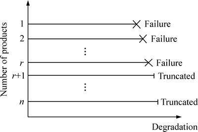
Fig. 2 Censored data of failure threshold

4.2 Updating RFT via EM algorithm

Generally, the estimation of RUL is primarily influenced by the mean value of RFT. Therefore, we only update the mean of RFT through the in situ data. For the lifetime estimation, it follows that Then, the TND can be approximated as traditional normal distribution, i.e. Suppose that the prior distribution of μ_w is normal distribution with mean μ_w0 and variance Based on the in situ data of failure threshold W_1:n, the posterior distribution of μ_w can be represented as follows.

                    (22)

Since the analytic form of Φ(·) does not exist, it is difficult to obtain the posterior However, the EM algorithm [42] provides a possible way for resolving this difficulty. The EM algorithm is an iterative procedure that repeatedly fills the missing data in the complete-data log-likelihood with their conditional expected values (E-step) and maximizes the complete data log-likelihood to update the parameter estimates (M-step) [43]. It has been widely used to find maximum likelihood or maximum posteriori estimation of parameters in statistical models, where the model depends on unobserved latent variables. Therefore, we use the EM algorithm to calculate the posterior

Let W_1:r={ω₁, ω₂, …, ω_r} represent the complete failure threshold data, and represent the real failure threshold of the remaining n-r products; then the complete log-likelihood function of can be written as follows.

 (23)

In sum, the EM algorithm consists of the following two steps.

1) E step:

Calculate

          (24)

For the censored data, the real failure threshold can be regarded to follow TND. That is, . Based on Eq. (2), we can obtain the expectation of as follows.

         (25)

2) M step:

Calculate  (26)

Take the first derivatives of the log-likelihood function in Eq. (24) gives

Calculate        (27)

By setting the above derivative to zero, can be expressed as

Calculate      (28)

Then, the E step and M step are iterated until a criterion of convergence is satisfied. The iteration is terminated using a standard criterion such as the difference between and falling below a pre-defined threshold. Note that maximizing Eq. (25) gives the mode of the posterior , which can be represented as Bayesian estimate of μ_w that minimizes the 0-1 loss function. Additionally, as the log-likelihood function in Eq. (23) is symmetric regarding μ_w, the mode of posterior is the mean. Therefore, the result of maximizing Eq. (25) is also the Bayesian estimate of μ_w that minimizes the mean quadratic loss function, which is commonly used as the Bayesian point estimation.

5 Numerical examples

In this section, we provide several numerical simulations to demonstrate that usefulness and application of the proposed models for an illustrative purpose. First, we compare the modelling of PRT with TDN with the traditional normal distribution. Then, the effort of RFT to RUL estimation and maintenance policy are demonstrated. Finally, the necessity of updating the RFT with the in situ failure threshold is proposed.

5.1 Mis-specification of RTF to RUL estimation

First, a numerical example is provided to show the deficiency in modelling the RFT by the traditional normal distribution. For illustrative purposes, the parameters for the degradation process are assumed as λ=1, μ_w=15, x_k=14, and where μ_w-x_k is small. Then, the corresponding PDFs and CDFs of the lifetime are illustrated in Fig. 3, where ND represents the traditional normal distribution. Obviously, the PDF and CDF by the traditional normal distribution are smaller than those by the TND. The reason can be explained as follows. When the traditional normal distribution is used to model the RFT, the PDF and CDF of RUL can be calculated by the law of total probability as follows.

                     (29)

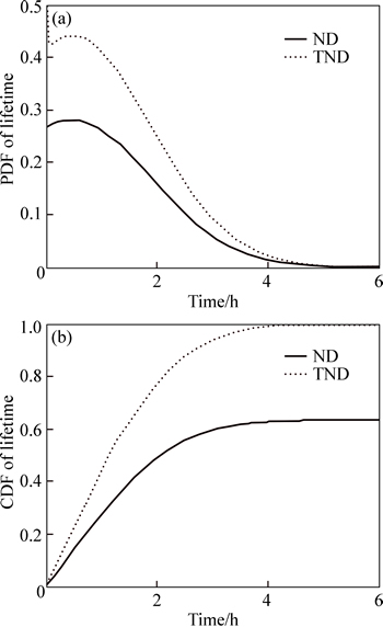
Fig. 3 Comparisons between estimated lifetime distributions with ND and TND

                     (30)

It can be observed that and are considered when the traditional normal distribution is used to model RFT. However, and will be negative since the integral is performed on condition that w-x_k>0. This is why the PDF and CDF derived via the traditional normal distribution are smaller.

5.2 Effect of RTF on lifetime estimation

In this experiment, a numerical example is provided to demonstrate the effect of the RFT on lifetime estimation. For an illustrative purpose, the parameters for the degradation process are assumed as λ=1, μ_w=10 and For simplicity, the model proposed in this work is referred to as M₀, and the model with a fixed threshold as M₁. Then, the corresponding PDFs and CDFs of the lifetime are illustrated in Fig. 4, where increases from 0.25 to 2.

It can be observed that the estimated lifetime is approximately unbiased but the variance of the estimated lifetime increases withThis is intuitively understandable since it is assumed that the RFT is independent of B(t) and thus the uncertainty of the degradation with the RFT is larger than that with a fixed failure threshold. In addition, the increase of first leads to the increase of the CDF and then leads to the decrease of the CDF. Furthermore, if a fixed threshold is utilized to estimate the RUL when the failure threshold is actually random, the failure probability in time zone [6, 9] would be underestimated and then the maintenance action may be delayed. Therefore, it increases the risk of failure.

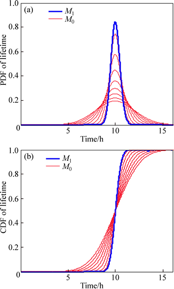
Fig. 4 Comparisons between estimated lifetime distributions with and without RFT

5.3 Effect of RTF on RUL estimation

To further illustrate the effect of the RFT on the estimated RUL, the case when μ_w increases with a fixed is presented in the follows. Figure 5 illustrates the compared results where and increases from 1, 8 to 15. It is shown that when decreases, the underestimated failure probability by using a fixed threshold to model the RFT increases. This is important for the maintenance policy based on the real time RUL estimation. It can be explained as follows. When more CM data are observed, the corresponding failure threshold (i.e. ) decreases. Therefore, it is necessary to model the RFT for the real time RUL estimation.

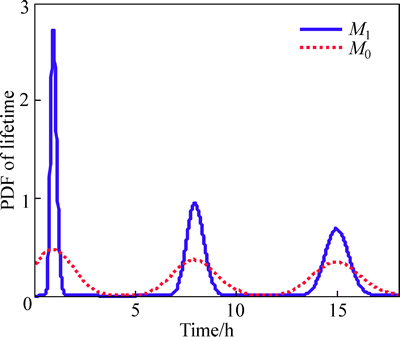
Fig. 5 Comparisons between estimated lifetime distributions with different μ_w

A numerical example is presented when the drift parameter of Wiener process is updated for RUL estimation. For illustrative purposes, the parameters for the degradation process are assumed as μ_λ=1, and Using these model parameters, 20 degradation paths are generated for deriving the initial estimated parameters which reflect the population-based degradation character, and 30 degradation paths are generated for evaluating the proposed method. The degradation paths are simulated by the Euler approximation method. The 30 degradation paths with measurement frequency of 1 h are illustrated in Fig. 6.

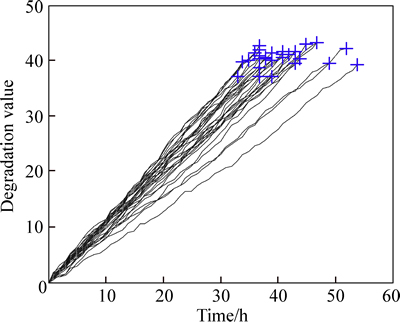
Fig. 6 Simulated degradation paths

The initial parameters are estimated by the maximum likelihood estimation method, and the results are μ_λ=1.017, and To evaluate the proposed method, the 2nd item is chosen to compare M₀ and M₁ at different CM times. As the actual threshold of item 2 is 38.41, the actual RUL can be approximately to be 36.8 based on the degradation path of item 2. For comparison, the corresponding PDFs of RULs under M₀ and M₁, and the actual RULs at t_k = 36 h are shown in Fig. 7. From Fig. 7, it can be observed that the range of the PDF of the RUL based on M₀ covers the actual RUL. However, the range of PDF of RUL based on M₁ does not cover the actual RUL. It can be observed that when the actual failure threshold is less than the defined threshold, the estimated RUL by M₁ is larger than the actual RUL and the PDF of the RUL could not cover the actual RUL. Thus, the maintenance is delayed which results in the failure before preventive maintenance.

Figure 8 shows the 95% confident interval (CI) of the RUL by M₀ and M₁ at some different CM points. For the CM time less than 25 h, the 95% CI of both models co observed, the corresponding failure threshold decreases. In this case, the underestimated failure probability by using a fixed threshold to model RFT increases. As a result, the 95% CI becomes narrower than that in the early CM times. This observation is consistent with the result derived by the above subsection.

ver the actual RUL. However, for the CM time more than 30 h, the 95% CI by M₁ does not cover the actual RUL. This implies that when more CM data are

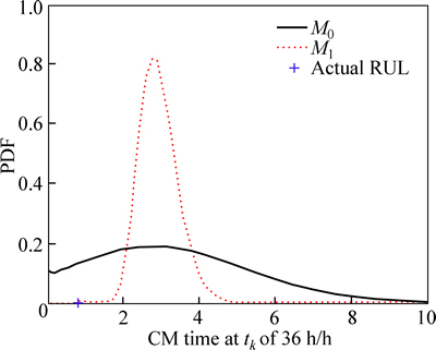
Fig. 7 Estimated PDFs of RUL by M₀ and M₁

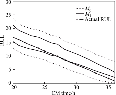
Fig. 8 95% confident interval of RUL by M₀ and M₁

5.4 Effects of RFT on maintenance policy

In order to give some insights to the influence of the RFT to replacement decision making, Eq. (21) is used to determine the replacement time. Let c_p=40 RMB and c_f= 100 RMB, then the expected cost per unit time at specific times is shown in Fig. 9. From Fig. 9, it can be observed that the decision by M₀ replaces the item at t_k = 34 h and the cost per unit time is 1.176 RMB/h. However, the decision by M₁ replaces the item at t_k=37 h while the item has already failed and the cost per unit time is 2.703 RMB/h. Obviously, using the RFT for the RUL estimation can avoid failure when the actual failure threshold is less than the estimated fixed failure threshold and thus the cost per unit time is reduced.

To further compare the influence to replacement decision making, the results based on the policy presented in Section 4.3 for all the 30 items are shown in Table 1, where the maintenance policies by M₀ and M₁ are respectively represented by Policy 0 and Policy 1, TC denotes the total cost, TOT denotes the total operating time and TCP denotes the total cost per unit time. It is clear that the replacement decision by M₀ results in a significantly lower cost per unit time. Although the decision by M₁ has a larger total operating time, it results in more FR and thus produces more cost.

5.5 Effects of updating RFT

This experiment compares the RUL estimation via the prior information of RFT with that via the updating RFT. Suppose that real model parameter of RFT are μ_w=10, and Suppose that the prior information of RFT is μ_w0=11, and The in situ failure thresholds data are displayed in Table 2, where the data of the first 5 items are the complete data, and the data of the last 5 items are the censored data. Based on the EM algorithm presented in Section 4, the posteriori of μ_w can be derived. The detailed iteration process is exhibited in Fig. 10. It can be observed that only after 10 iterations, the EM algorithm is converged. This implies that the EM algorithm could update the prior information of RFT efficiently. In this experiment, it is observed that the prior mean of RFT is 11, which is larger than the real value. If the wrong RFT is used, it could delay the maintenance time, cause failure maintenance, and decrease the system reliability and maintenance costs. However, after updating the RFT by the EM algorithm, the posteriori mean of RFT (10.02) is very close to the real value. It indicates the effectiveness of the EM algorithm.

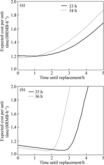
Fig. 9 Illustration of condition based replacement decision by M₀ and M₁

Table 1 Results of maintenance

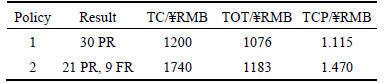
Table 2 In situ failure threshold data

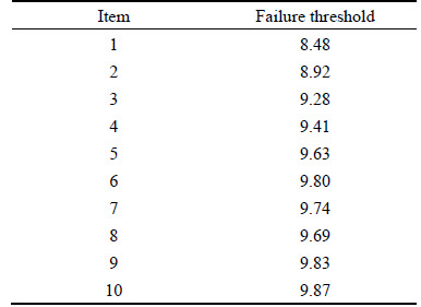
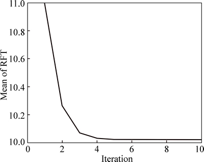
Fig. 10 Iteration process of μ_w

Overall, these simulations imply that the randomness of the failure threshold has significant effects on the real time RUL estimation and further on replacement decision making. The method proposed in this work can work well and efficiently. On the other hand, it is verified that considering the randomness of failure threshold and updating the prior information of RFT can improve the accuracy of the RUL estimation.

6 Conclusions

1) In this work, a Wiener based degradation process with RFT is proposed to estimate the PDF and mean of the RUL. Based on the characteristic of RFT, we use the TND to describe the RFT. By considering the randomness of failure threshold, an analytical mean and PDF of RUL is obtained in the sense of FHT considering the in situ CM data and uncertainty of the estimated drift parameter simultaneously. The analytical mean and PDF of RUL could simplify the calculation of the maintenance decision making.

2) Then, to improve the uncertainty of prior estimation of failure threshold, Bayesian method is used to update the prior estimation of failure threshold and EM is used to calculate the posteriori estimation of failure threshold.

3) Finally, several numerical examples are presented to illustrate the application and usefulness of the proposed method. It indicates that it is necessary to consider the uncertainty of failure threshold if it exists, and the prior estimation of failure threshold needs to be updated by the in situ failure data.

Primarily, it is discussed how to model the failure threshold by the normal distribution or TND. However, it is not limited to the normal distribution; other distributions could also be used to model RFT. And, if RFT is considered for the real time RUL estimation, its distribution should be truncated to satisfy the condition that the failure threshold should be larger than the current degradation. In addition, only the numerical examples are used to demonstrate the usefulness of the proposed method. Much more application in practice need to be further studied.

Appendix

The proof of Theorem 2:

As and it is easy to derive that From Lemma 3 and using the law of total probability, it can be obtained that

(A-1)

Let and the PDF of RUL can be obtained straightforwardly using Lemma 2.

From Theorem 1, the mean of RUL can be formulated as [9]

              (A-2)

This completes the proof.

References

[1] VAIDYA P, RAUSAND M. Remaining useful life, technical health, and life extension [J]. Proceedings of the Institution of Mechanical Engineers Part O: Journal of Risk and Reliability, 2011, 225(2): 219-231.

[2] LORTON A, FOULADIRAD M, GRALL A. Computation of remaining useful life on a physic-based model and impact of a prognosis on the maintenance process [J]. Proceedings of the Institution of Mechanical Engineers, Part O: Journal of Risk and Reliability, 2013, 227(4): 434-449.

[3] BO S, SHENGKUI Z, RUI K, PECHT M G. Benefits and challenges of system prognostics [J]. IEEE Transactions on Reliability, 2012, 61(2): 323-335.

[4] SI X, WANG W, HU C, ZHOU D. Remaining useful life estimation–A review on the statistical data driven approaches [J]. European Journal of Operational Research, 2011, 213(1): 1-14.

[5] CARR M J, WANG W. An approximate algorithm for prognostic modelling using condition monitoring information [J]. European Journal of Operational Research, 2011, 211(1): 90-96.

[6] WANG H, JIANG Y. Performance reliability prediction of complex system based on the condition monitoring information [J]. Mathematical Problems in Engineering, 2013, 2013: 1-7.

[7] WANG X L, JIANG P, GUO B, CHENG Z J. Real-time reliability evaluation based on damaged measurement degradation data [J]. Journal of Central South University, 2012, 19(11): 3162-3169.

[8] SI X, WANG W, HU C H, ZHOU D H, PECHT M G. Remaining useful life estimation based on a nonlinear diffusion degradation process [J]. IEEE Transactions on Reliability, 2012, 61(1): 50-67.

[9] PENG C, TSENG S. Mis-specification analysis of linear degradation models [J]. IEEE Transactions on Reliability, 2009, 58(3): 444-455.

[10] WANG X. Wiener processes with random effects for degradation data [J]. Journal of Multivariate Analysis, 2010, 101(2): 340-351.

[11] TANG S, GUO X, YU C, XUE H, ZHOU Z. Accelerated degradation tests modeling based on the nonlinear Wiener process with random effects [J]. Mathematical Problems in Engineering, 2014, 2014: 1-11.

[12] WANG W, CARR M, XU W, KOBBACY K. A model for residual life prediction based on Brownian motion with an adaptive drift [J]. Microelectronics Reliability, 2011, 51(2): 285-293.

[13] YE Z, TSUI K L, WANG Y, PECHT M G. Degradation data analysis using wiener processes with measurement errors [J]. IEEE Transactions on Reliability, 2013, 62(4): 772-780.

[14] TANG S, YU C, WANG X, GUO X, SI X. Remaining useful life prediction of Lithium-ion batteries based on the Wiener process with measurement error [J]. Energies, 2014, 7(2): 520-547.

[15] TANG S, GUO X, ZHOU Z. Mis-specification analysis of linear Wiener process–based degradation models for the remaining useful life estimation [J]. Proceedings of the Institution of Mechanical Engineers, Part O: Journal of Risk and Reliability, 2014, 228(5): 478-487.

[16] YE Z, SHEN Y, XIE M. Degradation-based burn-in with preventive maintenance [J]. European Journal of Operational Research, 2012, 221(2): 360-367.

[17] GEBRAEEL N Z, LAWLEY M A, LI R, RYAN J K. Residual-life distributions from component degradation signals: A Bayesian approach [J]. IIE Transactions, 2005, 37(6): 543-557.

[18] YE Z, CHEN N, TSUI K L. A Bayesian approach to condition monitoring with imperfect inspections [J]. Quality and Reliability Engineering International, 2015, 31(3): 513-522.

[19] WANG X, GUO B, CHENG Z. Residual life estimation based on bivariate Wiener degradation process with time-scale transformations [J]. Journal of Statistical Computation and Simulation, 2012, 84(3): 1-19.

[20] SI X, WANG W, HU C, ZHOU D. Remaining useful life estimation– A review on the statistical data driven approaches [J]. European Journal of Operational Research, 2011, 213(1): 1-14.

[21] WANG X, JIANG P, GUO B, CHENG Z. Real-time reliability evaluation with a general wiener process-based degradation model [J]. Quality and Reliability Engineering International, 2014, 30(2): 205-220.

[22] TANG S, GUO X, YU C, ZHOU Z, ZHOU Z, ZHANG B. Real time remaining useful life prediction based on nonlinear Wiener based degradation processes with measurement errors [J]. Journal of Central South University, 2014, 21(12): 4590-4517.

[23] WANG X, BALAKRISHNAN N, GUO B. Residual life estimation based on a generalized Wiener degradation process [J]. Reliability Engineering & System Safety, 2014, 124: 13-23.

[24] XU Z, JI Y, ZHOU D. Real-time reliability prediction for a dynamic system based on the hidden degradation process identification [J]. IEEE Transactions on Reliability, 2008, 57(2): 230-242.

[25] FENG L, WANG H, SI X, ZOU H. A State-space-based prognostic model for hidden and age-dependent nonlinear degradation process [J]. IEEE Transactions on Automation Science and Engineering, 2013, (10)4: 1072-1086.

[26] WANG X, GUO B, CHENG Z, JIANG P. Residual life estimation based on bivariate Wiener degradation process with measurement errors [J]. Journal of Central South University, 2013, 20(7): 1844-1851.

[27] WANG P, COIT D W. Reliability and degradation modeling with random or uncertain failure threshold [C]// Proceedings of the Reliability and Maintainability Symposium, 2007 RAMS '07 Annual. Orlando, FL: IEEE, 2007: 392-397.

[28] WANG W. A two-stage prognosis model in condition based maintenance [J]. European Journal of Operational Research, 2007, 182(3): 1177-1187.

[29] WEI M, CHEN M, ZHOU D. Multi-sensor information based remaining useful life prediction with anticipated performance [J]. IEEE Transactions on Reliability, 2013, 62(1): 183-198.

[30] ZIO E, COMPARE M. Evaluating maintenance policies by quantitative modeling and analysis [J]. Reliability Engineering & System Safety, 2013, 109: 53-65.

[31] USYNIN A, HINES J W, URMANOV A. Uncertain failure thresholds in cumulative damage models [C]// Proceedings of the Reliability and Maintainability Symposium, 2008 RAMS 2008 Annual. Las Vegas: IEEE, 2008: 334-340.

[32] JIANG R, JARDINE A K S. Health state evaluation of an item: A general framework and graphical representation [J]. Reliability Engineering & System Safety, 2008, 93(1): 89-99.

[33] JIANG R. A multivariate CBM model with a random and time-dependent failure threshold [J]. Reliability Engineering & System Safety, 2013, 119: 178-185.

[34] GREENE W H. Econometric analysis [M]. 5th Ed, Upper Saddle River. New Jersey: Prentice Hall, 2003: 756-760.

[35] FOLKS J L, CHHIKARA R S. The inverse gaussian distribution and its statistical application-A review [J]. Journal of the Royal Statistical Society Series B: Methodological, 1978, 40(3): 263-289.

[36] SI X, WANG W, CHEN M, HU C, ZHOU D. A degradation path-dependent approach for remaining useful life estimation with an exact and closed-form solution [J]. European Journal of Operational Research, 2013, 226(1): 53-66.

[37] SI X, WANG W, HU C, CHEN M, ZHOU D. A Wiener-process- based degradation model with a recursive filter algorithm for remaining useful life estimation [J]. Mechanical Systems and Signal Processing, 2013, 35(1/2): 219-237.

[38] ZHOU Z, HU C, YANG J, XU D, ZHOU D. Online updating belief-rule-base using the RIMER approach [J]. IEEE Transactions on Systems, Man and Cybernetics, Part A: Systems and Humans, 2011, 41(6): 1225-1243.

[39] YOU M, LIU F, WANG W, MENG G. Statistically planned and individually improved predictive maintenance management for continuously monitored degrading systems [J]. IEEE Transactions on Reliability, 2010, 59(4): 744-753.

[40] CADINI F, ZIO E, AVRAM D. Model-based Monte Carlo state estimation for condition-based component replacement [J]. Reliability Engineering & System Safety, 2009, 94(3): 752-758.

[41] G, GALANTE G, LOMBARDO A. A predictive maintenance policy with imperfect monitoring [J]. Reliability Engineering & System Safety, 2010, 95(9): 989-997.

[42] DEMPSTER A P, LAIRD N M, RUBIN D B. Maximum likelihood from incomplete data via the EM algorithm [J]. Journal of the Royal Statistical Society Series B: Methodological, 1977, 39(1): 1-38.

[43] YE Z, NG H K T. On analysis of incomplete field failure data [J]. The Annals of Applied Statistics, 2014, 8(3): 1713-1727.

(Edited by FANG Jing-hua)

Foundation item: Projects(51475462, 61174030, 61473094, 61374126) supported by the National Natural Science Foundation of China

Received date: 2015-04-09; Accepted date: 2015-06-11

Corresponding author: YU Chuan-qiang, PhD, Associate Professor; Tel: +86-29-84741547; E-mail: yuchuanqiang201@126.com