J. Cent. South Univ. (2020) 27: 114-131

DOI: https://doi.org/10.1007/s11771-020-4282-5

A novel shapelet transformation method for classification of multivariate time series with dynamic discriminative subsequence and application in anode current signals

WAN Xiao-xue(万晓雪), CHEN Xiao-fang(陈晓方), GUI Wei-hua(桂卫华),YUE Wei-chao(岳伟超), XIE Yong-fang(谢永芳)

School of Automation, Central South University, Changsha 410083, China

Central South University Press and Springer-Verlag GmbH Germany, part of Springer Nature 2020

Abstract: Classification of multi-dimension time series (MTS) plays an important role in knowledge discovery of time series. Many methods for MTS classification have been presented. However, most of these methods did not consider the kind of MTS whose discriminative subsequence was not restricted to one dimension and dynamic. In order to solve the above problem, a method to extract new features with extended shapelet transformation is proposed in this study. First, key features is extracted to replace k shapelets to calculate distance, which are extracted from candidate shapelets with one class for all dimensions. Second, feature of similarity numbers as a new feature is proposed to enhance the reliability of classification. Third, because of the time-consuming searching and clustering of shapelets, distance matrix is used to reduce the computing complexity. Experiments are carried out on public dataset and the results illustrate the effectiveness of the proposed method. Moreover, anode current signals (ACS) in the aluminum reduction cell are the aforementioned MTS, and the proposed method is successfully applied to the classification of ACS.

Key words: anode current signals; key features; distance matrix; feature of similarity numbers; shapelet transformation

Cite this article as: WAN Xiao-xue, CHEN Xiao-fang, GUI Wei-hua, YUE Wei-chao, XIE Yong-fang. A novel shapelet transformation method for classification of multivariate time series with dynamic discriminative subsequence and application in anode current signals [J]. Journal of Central South University, 2020, 27(1): 114-131. DOI: https://doi.org/10.1007/s11771-020-4282-5.

1 Introduction

Multi-dimension time series (MTS) are widely used in many areas such as speech recognition, multimedia, medicine, economics, science and engineering [1, 2]. MTS classification plays an important role in knowledge discovery of time series [3]. Therefore, a large number of researches have been performed and several methods have been presented for MTS classification [3-5]. A simple method combining 1-nearest neighbor rule (1NN) with dynamic time warping (DTW) was proposed in Refs. [6, 7]. However, the interpretability is hardly presented in 1NN because there are only information about similarity between two time series. Moreover, due to the time and space complexity, the application of this method is limited [8]. Most of these approaches are defined as features extracting [9, 10]. In these studies, many features extracted from MTS were expected to replace the original MTS. The advantage of these methods is avoiding dimension curse with the reduction of dimension and the length of MTS samples [11].

Mining core features for early classification was used to classify time series [1]. The core features were obtained by clustering candidate shapelets in each dimension for one class sample. Another method called multi-dimension shapelets detection (MSD) classifies MTS by extracting multi-dimension shapelets [12]. Each shapelet in multi-dimension shapelets was extracted from one dimension. Most of the MTS classification methods did great researches for MTS. However, they often extracted features by comparing the same dimension signal. Therefore, they didn’t take into consideration of a kind of MTS whose discriminative subsequence is not restricted to dimension [13]. In other words, the method which extracts feature in each dimension may be invalid for MTS when its dimensions are not typically independent and identically distributed.

Shapelet transformation is one of the most successful algorithms for unidimensional time series (UTS) classification with high accuracy for amount of time series data mining in classification [14], clustering [15, 16], summarization [17, 18] and visualization [19, 20]. Shapelet is a subsequence or shape, and it is a representative feature for one class. By finding the best k shapelets in n time series with a single-scan algorithm, the transformed data combining with classifiers preformed a greater accuracy which was proved in Ref. [21]. The great advantage of shapelet transformation is that it can match discriminative subsequences unlimited to the structure of data [22]. However, most of the shapelet transformation work is about classifying UTS. Though there are few extended shapelet transformations to MTS [11, 23], all of them extract shapelets from different and independent dimensions [24, 25]. For example, in industrial datasets, the feature of anode current signals (ACS) in one dimension standing for a class also likely appeared in other dimensions [23].

In this work, in order to overcome the limitations of the existing shapelet transformation, an extended shapelet transformation method is proposed to classify MTS with discriminative subsequence and without restrictions to dimension. Firstly, for original shapelet transformation, k shapelets are extracted from UTS and transformed into distance. Too many shapelets may lead to over-fitting on training set and reducing influence of the most interpretable shapelets [26]. Therefore, to reduce the number of shapelets and overcome the restrictions of dimension with discriminative subsequence, k shapelets are replaced by key features which are extracted from candidate shapelets with one class for all variables. Secondly, taking consideration of the influence of feature number on accuracy, a feature of similar numbers is proposed, which stands for the frequency of a key feature appearing in a multi-dimension time series. Based on the proposed method, the signals whose discriminative subsequence is not restricted to dimension will be classified well. Thirdly, exhaustive search of shapelets is time-consuming and clustering shapelets adds the time complexity [27, 28]. To reduce the time complexity, distance matrix is used to calculate the distance between shapelet and time series. Because the calculations between shapelet and time series have many repetitions, the amount of computation can be reduced by calculating ahead. Distance matrix was created to group similar shapelets in Ref. [21]. In this way, distance matrix not only clusters similar shapelets but also reduces the time complexity.

The paper is organized as follows. In Section 2, the background is provided. In Section 3, our method is proposed and developed. In Section 4, the experiments are performed on common datasets and ACS datasets, and also the discussions are presented. Finally, in Section 5 the conclusions and future work are given.

2 Background

2.1 Related definitions

In this section, related definitions and notations for MTS classification are given.

Definition 1: Unidimensional time series: T=(t₁, t₂, …, t_N) is a sequence of values which are recorded in temporal order. The number of the values in T standing for the length of T is N.

Definition 2: Multi-dimension time series: M=(T₁, T₂, …, T_r) is a vector of UTS T_i. The dimension of M is r. For datasets M^w, each MTS M_i relates to a class label The number of datasets is w, and the number of categories is q. The task of time series classification is mapping an unknown MTS M_i to a class label c_i∈C.

Definition 3: Subsequence: b=(t_m, t_m+1, …, t_(m-l)+1) is a contiguous value belonging to T, which starts at the m-th point and ends at the ((m-l)+1)-th point with length l. As shown in Figure 1(a), S₁ is a subsequence in UTS T₁. A UTS T=(t₁, t₂, …, t_N) contains (N-l)+1 subsequences of length l. As MTS M=(T₁, T₂, …, T_r) has r UTS, the number of subsequence in M is r×((N-l)+1). The subsequence is used for creating candidate shapelets.

Definition 4: Euclidean distance(ED): the similarity measurement of two subsequences b=(e₁, e₂, …, e_l) and p=(d₁, d₂, …, d_l) of length l. The ED between subsequences b and p is calculated by computing each point between b and p by siding window. The computational formula is below:

                   (1)

Eq. (1) illustrates that the smaller the dist(b, p), the more similar the b and p.

Definition 5: Distance between subsequences b and UTS: the similarity measurement of a subsequences b and UTS Calculate the distance between b and T with Eq.(2):

               (2)

where S_i is the i-th subsequence of T by sliding window of length |b|. As shown in Figure 1(a), the distance between subsequences b and UTS T₁ equals the least distance between subsequences b and S_i, which is a candidate shapelet in T₁. In Figure 1(a), the candidate shapelet in T₁ is S₁.

Definition 6: Distance between subsequences b and MTS: the similarity measurement of a subsequence b and a MTS M=(T₁, T₂, …, T_r). M consists of UTS T_i. The formula is illustrated by Eq.(3):

              (3)

where is defined in Eq. (2), and the purpose to calculate the distance is to find the most similar subsequence of b in a MTS. As shown in Figure 1, for MTS M with 3 variables, we can see that the subsequence b maps each UTS in dimension for M, respectively. The most similar subsequence of b in M is S₁ as shown in Figure 1(a). The distance between sequence S₁ and b is calculated with Eq. (1).

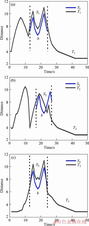
Figure 1 Distance between subsequence b and MTS M

Definition 7: Distance set: a set of distances between subsequence b and MTS M_i of datasets M^w. The number of datasets is w. The distance set is:

                          (4)

Definition 8: Split point(sp): a real number to split the ordered distance set into two sets and The set of sp is (sp₁, sp₂, …, sp_n). For distance set O, sp_j in sp set is calculated by Eq. (5):

                            (5)

where sp_j with the highest information gain is recorded as the best sp, which is used to split datasets lastly. The value of the best sp also calls as threshold.

Definition 9: Information gain (IG): the standard of assessment quality of shapelets. A distance set O is divided by a sp into O_L and O_R. The distance of O_L is less than sp, and it is the contrary to O_R. For each sp, IG is calculated as follows:

(6)

We get the best IG by comparing all of the IG with every sp in sp set. The H(O) is calculated in Eq.(7).

Definition 10: Entropy: the complexity of datasets. For a datasetthe class of datasets is e_i is the number of samples for class c_i . Entropy of P is calculated as below:

                       (7)

2.2 Problem description of MTS with dynamic discriminative subsequence

Generally speaking, all MTS belonging to one class always have the same characteristic. The characteristic is defined as discriminative subsequence in our method. There is a kind of MTS whose discriminative subsequence is not restricted to dimension. We call this kind of MTS as MTS with dynamic discriminative subsequence. In the aluminum reduction industry, ACS which can reflect the distributed aluminum reduction cell condition, is a kind of MTS with dynamic discriminative subsequence, is illustrated in Example 1.

Example 1: Two 4-dimensional MTS objects that have the same key feature for ACS are shown in Figure 2. Signals shown in Figures 2(a)-(d) are extracted from the same MTS(M₁), the same as signals shown in Figures 2(e)-(h) which are extracted from M₂, and M₁ and M₂ belong to the same class. Signals (a) and (e) belong to dimension a. In the same way, signals (b) and (f) belong to dimension b. Assuming that a discriminative subsequence for time series M₁ is extracted in dimension a shown in Figure 2(a) and it is extracted in dimension c for time series M₂ shown in Figure 2(g). To sum up, the discriminative subsequence standing for the same class isn’t extracted in one fixed dimension. As a result, the ACS is different from common MTS which has the same feature in each dimension of the same class. It’s difficult to classify this kind of MTS with common classification method.

3 Extracting features with extended shapelet transformation (EFEST)

In this section, an approach to extract new features with extended shapelet transformation is proposed, as shown in Figure 3. Firstly, candidate features are extracted by siding window. Secondly, a distance matrix is built by candidate shapelets. By sorting the quality of candidate shapelets using distance matrix, shapelets are selected with the highest quality in a dimension. This is the first step to extract shapelets by distance matrix. In the next step, key features without the restriction of dimensionality are extracted from shapelets by clustering. In the last step, a feature of similarity numbers is added into transformed data to classify; the feature of similarity numbers and key features are translated into distance against original data. The data of distance will be trained into classifier.

3.1 Extracting shapelets by distance matrix in MTS

Unlike MSD, we extract all candidate shapelets in all dimension of a MTS. Firstly, after datasets M^w have been normalized, candidate shapelet is extracted in each dimension as a subsequence with length l between l_min=3 and l_max=N. As shown in Figure 4, candidate shapelets are extracted by sliding window in every dimension of MTS. T_i is one of the variable in a MTS. For a UTS (N-l+1) candidate shapelets can be extracted. For a MTS M=(T₁, T₂, …, T_r), the number of candidate shapelets is r×((N-l)+1). Therefore, a datasets M^w contains w×r×((N-l)+1) candidate shapelets.

After extracting candidate shapelets, we use the candidate shapelets to build a distance matrix (line 13 of Algorithm 1). The matrix is constituted by the distance between each pair of candidate shapelets. In the previous step, (w×r×(N-l+1)) candidate shapelets have been extracted. Therefore, the size of distance matrix is (w×r×(N-l+1))× (w×r×(N-l+1)). The matrix element i×j is the distance between the i-th candidate shapelet and the j-th candidate shapelet. The distance matrix is symmetry by the diagonal. An example of distance matrix is shown in Figure 5. C_i is the name of a candidate shapelet. The value of coordinates calculated by Eq. (1). (C₁, C₂) is the distance between candidate shapelets C₁ and C₂. All of the values are symmetry by the diagonal. Because half of the distance between candidate shapelets is calculated repeatedly, the complexity of calculating can be reduced on half by duplicating.

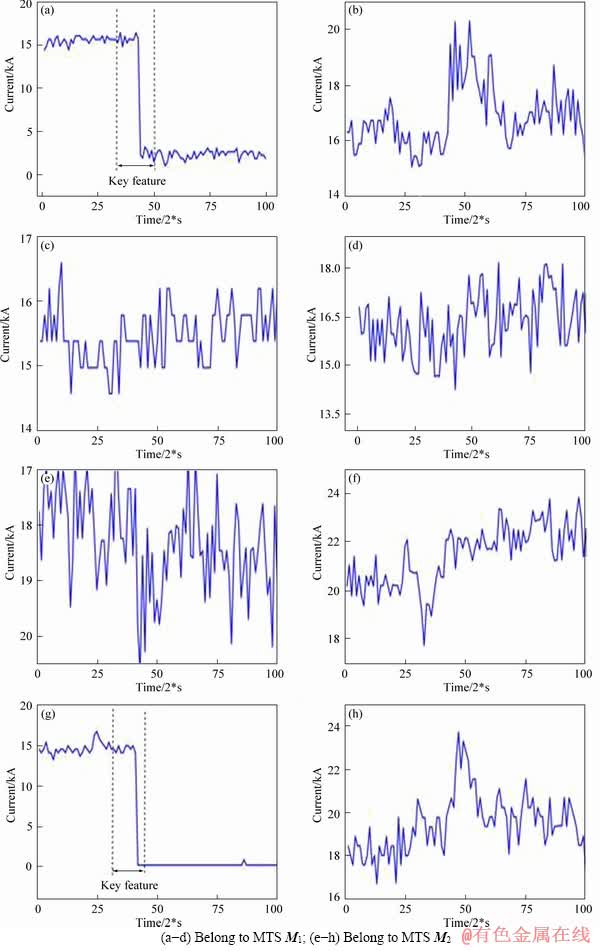
Figure 2 Two 4-dimensional MTS objects:

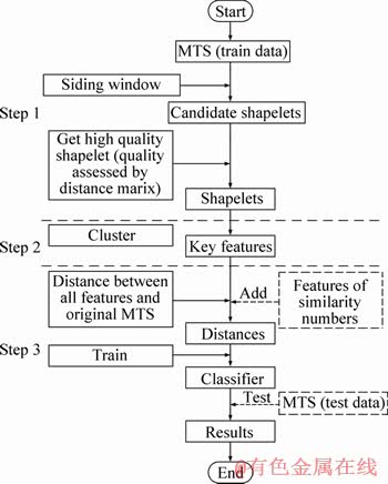
Figure 3 Flowchart of extracting features with extended shapelet transformation

Figure 4 Illustration of extracting candidate shapelets in MTS

Distance matrix is only used to cluster shapelets in the existing researches [21]. In this method, distance matrix is used to calculate the distance between candidate shapelets and MTS (line 15 of Algorithm 1). As candidate shapelets are extracted in UTS by sliding window, a UTS is made up of candidate shapelets. At the same time, the MTS consist of candidate shapelets. To calculate the distance between a candidate shapelet and MTS, the length of MTS is pre-computed. After we find the candidate shapelets in the range of the length, the distance between a candidate shapelet and MTS is the smallest between the candidate shapelet and candidate shapelets in MTS. For example, in Figure 5, each M_i of the datasets M^w has n candidate shapelets. The distance between C₁ and M₁ which consist of n candidate shapelets is the smallest between C₁ and candidate shapelets in M₁.

Algorithm 1 Extracting features

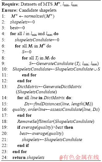
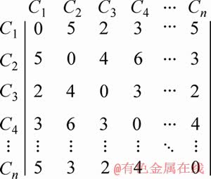
Figure 5 A example of distance matrix

The last step is to assess the candidate shapelets by information gain (line 16 of Algorithm 1). A distance set of distance between sequence b and datasets M^w is built in Eq. (4). We use a sp to split distance set into two subsets. The split is chosen in the set of sp with the highest information gain. For instance, the sp set of distance set O₁=(d₁, d₂, …, d_w) is (sp₁, sp₂, …, sp_n). The value of sp is calculated by Eq. (5). After the information gain of each sp is calculated by Eq. (6), we suppose that the optimal sp named sp₂ is got with the highest information gain. The value of sp₂ is recorded as threshold. The information gain is recorded as quality. Therefore, we get the quality of each candidate shapelet. To choose the most representative sequence, we remove the self-similarity candidate shapelets (line 18 of Algorithm 1). In other words, a shapelet in a UTS with the highest quality is chosen (lines 19-21 of Algorithm 1). Accordingly, only one shapelet is extracted from a UTS. In the end, the shapelet set for different length of shapelet with the highest average quality is retained. For datasets M^w, there are r_*w shapelets .

3.2 Extracting key features without restriction of dimensionality

To classify the kind of MTS with dynamic discriminative subsequence, we mine key features in MTS in one class by clustering with distance matrix. Firstly, if shapelets have high quality in a class, they are always more similar than other shapelets. Consequently, it’s necessary to extract high quality as key features which discriminate classes well. Secondly, by calculating the distance between key features and each sample in MTS dataset, the dataset will be well gathered, which can increase the accuracy of classification. In Algorithm 2, the first step is to delete self-similar candidate shapelets in distance matrix coordinate to retain valid shapelets (line 1 of Algorithm 2). For the k valid shapelets in one class, this is a k×k matrix. The element in distance matrix stands for the distance between each pair of valid shapelets. The clustering process is based on updated distance matrix (lines 2-9 of Algorithm 2). As the smallest value is 0 which is the distance between the same candidate shapelets. The smallest distance between different candidate shapelets is the second small value. Firstly, the pair with the second small shapelet distance between them is clustered. Secondly, the clustered pair is removed and cluster is added into matrix. The k×k matrix is changed into (k-1)×(k-1) matrix. The distance between each shapelet and the cluster is the average distance between the shapelet and every shapelet in cluster. After updating the distance matrix, we repeat the process above until all of the shapelets have been clustered, and then we get several clusters in the end. For shapelets in each cluster, the highest quality shapelet is selected as a key feature.

Algorithm 2 Extracting key feature

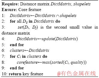
Example 2: An example for the process of clustering shapelets based on distance matrix is illustrated in Figure 6. A distance matrix D consisting of shapelets is shown in Figure 6(a). S_i is the name of valid shapelets. In the next step, 1 is founded as the second small value in D. 1 is the distance between shapelet S₁ and S₂ in Figure 6(b). Therefore, shapelets S₁ and S₂ are the most similar shapelet pair in D. We replace S₁ and S₂ by the cluster of S₁ and S₂ shown in Figure 6(c). The distance between shapelet S₃ and cluster of (S₁, S₂) is the average distance between S₃ and (S₁, S₂). The process is repeated until all of the shapelets are clustered.

Figure 6 A process of clustering base on distance matrix D

3.3 A novel feature: feature of similarity numbers extracted

In this section, we propose an algorithm to transform data with key features. The advantage of shapelet transformation is that the data transformed into distance can be used in many classifiers. The distance between key features and sample in raw datasets is calculated. However, it can’t perfectly represent the raw datasets, and Example 3 is presented to illustrate this.

Example 3: Two 4-dimensional MTS are shown in Figure 7. They have the same dimensions of a, b, c and d. MTS A with class anode effect (AE) is composed of UTS a₁, b₁, c₁ and d₁. After being clustered, a kind of key feature is extracted in red line. In Figures 7 (e)-(h), another MTS B where d₂ has the same key feature like Figures 7(a)-(d) is marked as normal. The feature trained by classifier is the minimum distance between the key feature and four UTS shown in Figure 7. The MTS A and B almost have the same distance to key features. As a result, we can conclude that the key features can’t identify the MTS with one key feature and MTS with multiple key features.

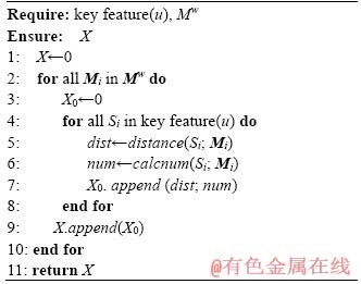
To solve the problem in Example 3, feature of similarity number is added to complete the algorithm. In Algorithm 3, firstly, for each instance in datasets M^w, we find the distance between M_i and each key feature (line 5 of Algorithm 3). Secondly, for each key feature, the number of the distance between each UTS in a instance and key feature less than the threshold is counted. For example, MTS M₁=(T₁, T₂, …, T₁₀), T_i in M₁ is a UTS. Suppose that the distance between key feature C and T_i in M₁ is (3.1, 4.2, 4.2, 3.5, 5.6, 6.7, 2.1, 3.4, 2.3, 3.0). The optimal sp selected from sp set with the highest information gain of key feature is 3. If the distance less than threshold, the time series are similar. Therefore, key feature has similar sequence in T₇ and T₉. In other words, key feature is similar to UTS T₇ and T₉ because the distance 2.3 is less than 3. The number of UTS which is similar to key feature in this example of 2, is marked as the feature of similarity numbers. We add the feature of similarity numbers into transformed data made up of the distance between key features and original data. If the number of key feature is u, the transformed data are a matrix with u columns. Because the number of key features equals the number of features of similarity number, the transformed data added feature are a matrix with 2×u columns different from u columns. Finally, the data are classified by traditional classifier.

Algorithm 3 Transforming data based on key feature

4 Experimental results and discussion

In this section, we give an empirical evaluation of our proposed method in common datasets and ACS datasets. To prove the superiority of our method, we compare our method with an extension of original shapelet transformation to MSD method,the hidden-unit logistic model (HULM) method [29] and shapelet ensemble for multi-dimensional time serie (SEMTS) method [30]. And then, feature of similarity numbers and distance matrix are tested to verify the effectiveness. The comparison of classifiers can find the best classifier for our method. This experiment follows a 10-fold cross-validation scheme with each 4-time running. At last, we take the average results. We get the results using a PC computer with Intel Core 3.7 GHZ and 8 GB of main memory. The length of candidate shapelets is between l_min=3 and l_max=L/4 (L is the full length of time series). The algorithms are implemented in Python using Spyder2.7.

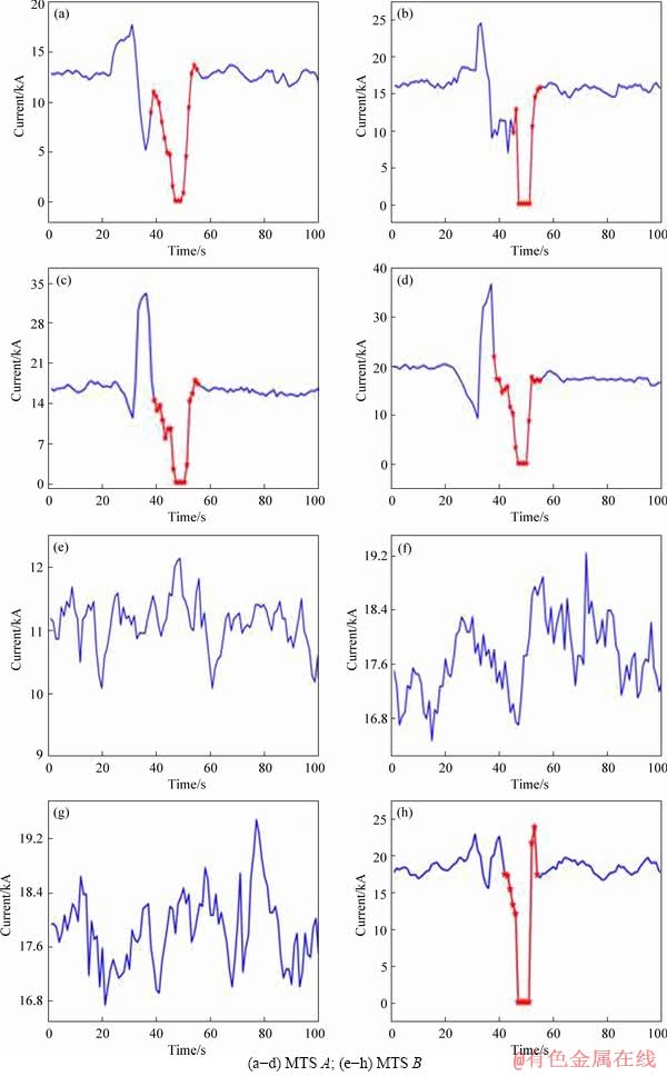
Figure 7 Two 4-dimensional MTS having same dimensions of a, b, c and d:

4.1 Numeric test on benchmark

4.1.1 Datasets and data preprocessing

We select seven common datasets to support the proposed approach. The datasets are Robot failure LP1, Robot failure LP3, Robot failure LP4, Wafer, Australian sign language signs, Japanese vowels and ECG. The Robot failure LP1, Robot failure LP3 and Robot failure LP4 are in small size. The Robot failure LP1 has 88 samples with 4 classes; Robot failure LP3 has 47 samples with 4 classes; Robot failure LP4 has 117 samples with 3 classes. The length of Robot failure LP1, Robot failure LP3 and Robot failure LP4 are 15, and the variables are 6. Wafer, Australian sign language signs, Japanese vowels and ECG are in big size. Wafer has 1194 samples, 198 of max length and 6 variables; Australian sign language signs has 2565 samples, 136 of max length and 22 variables. Japanese vowels has 640 samples, 640 of max length and 126 variables; ECG has 200 samples, 152 of max length and 2 variables. We randomly split the samples into training set and test set. The datasets details are gathered in Table 1 [18].

We carry out a data preprocessing process before calculating the distance between candidate shapelets. The preprocessing method is different from the existing methods [11] which normalize linearly the value in the same variable. We normalize linearly all of the data by zero-mean normalization shown in Eq. (8):

                             (8)

where x_mean and v are the mean and variance for all samples, respectively. The mean and variance of preprocessed data are 0 and 1. Preprocessing can avoid the big wave of the signal dominate the small wave of the signal, which keeps the rationality of comparing with ED effectively.

Table 1 Detail information of common datasets

4.1.2 Experimental results and analysis

Our method is compared with MSD, HULM and SEMTS method. MSD extracted a multi-dimension shapelets S_j=(s₁^(j), s₂^(j), …, s_r^(j)) which consist of multiple shapelets extracted from each dimension [12], and r is the dimension of MTS. It’s used for early classification before. We extend MSD method to shapelet transformation to compare with our method. The distance between shapelet vector and M_i=(T₁⁽ⁱ⁾, T₂⁽ⁱ⁾, …, T_r⁽ⁱ⁾) is a vector of distance corresponding with dimension and it’s calculated by Eq. (9):

                         (9)

whereis used to compare the similarity between shapelet vector and MTS. If sum(dist(S₁, M₂)) is smaller than sum(dist(S₂, M₂)), the vector of shapelets S₁ is more similar to M₂ than S₂. For the method of extending shapelets transformation to MSD, shapelet is replaced by shapelet vector, and the distance between shapelet and UTS is replaced by sum(dist(S_j, M_i)). In this case, we change the MTS classification question into a UTS classification question. As MSD can only compare with datasets whose dimensions are in same length, we just use dataset Robot failure LP1, Robot failure LP3 and Robot failure LP4 by comparison.

HULM uses binary stochastic hidden units to latent structure in the data. Comparing to the prior models temporal dependencies in the data, the advantage of HULM is that it can model very complex decision boundaries.

SEMTS proposed a shapelet discovery technique that allows efficient candidates evalua tion in multivariate time series forest. It’s the first attempt to generalize shapelet discovery to multi- dimensional time series by teaming up a set of decision trees based on majority vot ing. After generating a set of tree in each dimension, it classified each dimension and chose the highest accuracy of each dimension as final accuracy. The code is available in Ref. [30].

Extreme gradient boosting (XGBoost) classifier is used for all of the experiments. The results of the comparison between MSD, EFEST- XGBoost, HULM and SEMTS method are gathered in Table 2 and Figure 8. It is clear that the EFEST method is more accurate than MSD, HULM and SEMTS method. For each common data, our method has better accuracy in total. More particularly, the accuracy based on our method for Robot failure LP4 is 100%. Comparing with the MTS in the same dimension, MSD didn’t consider the relationship of dimensions. Moreover, the shapelets in shapelet vector are all in the same location. When the length of time series is in different dimensions, MSD method is invalid. For our method, the key feature which is used to translate into distance has no restrictions of dimension and location.

Table 2 Accuracy comparison of different method

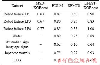
Therefore, the highest quality of subsequence can be extracted. SEMTS method makes an assumption that individual dimensions are independent. It didn’t consider the relevance of dimensions. The multi-length indexing of SEMTS method is used to reduce the computation, and it has no change in accuracy due to skipping some of the length. For almost all of the datasets, our method is better than HULM. Though the performance of two methods is quite similarly, the interpretability of our method is better than HULM. Shapelets extracted by our method are comprehensible and can offer insight into the problem domain. By drawing the dot of shapelets, the key wave feature can be seen. To sum up, the advantage of our method is decreasing the influence of dimension to extracted features. In addition, clustering shapelets, which reduces the number of shapelets, will increase interpretability of shapelets. Though our method is based on a special kind of MTS, the experiments illustrate that our method apply equally to common datasets and the study on MTS’s structure is meaningful.

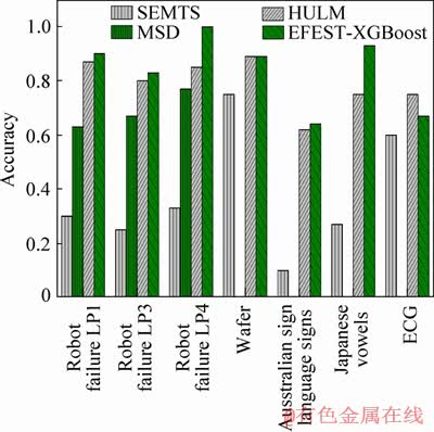
Figure 8 Accuracy comparison of different methods

Table 3 Testing accuracy of complex classifiers

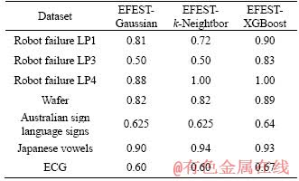
Classifying the transformed data is the second important step to complete algorithm. A useful classifier can increase the accuracy sharply. We compare the precision rate based on classifiers XGBoost, k-Nearest Neighbor and Naive Bayes. XGBoost is based on gradient boosting which is in terms of systems optimization and principles in machine learning. With great improvement, regularization is added to loss function in XGBoost to establish the objective function and avoid overfitting [13]. The naive Bayes classifier greatly simplifies learning by assuming that features are independent on given class [31]. Although independence is generally a poor assumption, in practice, Naive Bayes often shows the accuracies for classifier XGBoost, k-Nearest Neighbor and Naive Bayes on common data. The Gaussian has the worst accuracy on average, and XGBoost classifier has great advantage than other two classifiers. To sum up, our method combining with XGBoost shows excellent accuracy.

We add feature of similarity numbers to train data. In this section, Table 4 presents the accuracies of XGBoost, k-Neighbor and Gaussian on transformed data added feature of similarity numbers. For the datasets Robot failure LP3, Robot failure LP4, Wafer, Australian sign language signs, Japanese vowels and ECG, adding feature has no advantage to accuracy. For the datasets Robot failure LP1, adding feature is more precise than without adding feature based on XGBoost and Guassian classifier. To conclude, the accuracy of adding feature method is influenced by data type and classifier. One possible reason is that different data types have different responds to feature of similarity numbers. If the number of subsequences, which is similar to key features in time series, has no influence to class, adding features is invalid. The possible reason of the less precise of adding feature based on k-Neighbor classifier is that k-Neighbor needs mass samples.

Table 5 presents the running time of extracting features based on MSD method and EFEST. The running time of generating distance matrix is recorded for EFEST. At the same time, we record the time of creating candidate shapelets for MSD method. For common datasets Robot failure LP1, the running time is 53 s for distance matrix, and it takes more 11 s than MSD method. For common datasets Robot failure LP3 and LP4, they take 14 and 102 s for distance matrix, respectively. However, they take only 10 and 67 s for MSD, respectively. The results show that our method has a bad performance to reduce time complexity in small size common data. It is possible that distance matrix is supposed to reduce the calculate amount by duplication. For small data set, duplication costs more running time than calculation. For big datasets of Wafer, Australian sign language signs, Japanese vowels and ECG, because the length of UTS is long, the variable and the sample number are multiple, distance matrix has better performance with reducing running time almost on half. The reason is that calculation takes much more time than duplication for big datasets. Distance matrix can replace calculation by duplication on half. Therefore, the running time can be reduced on half almost.

4.2 Application in anode current signals

4.2.1 Analysis of anode current signals

Aluminum reduction cell, here after referred to as the cell, is characterized by coupling,randomness, multivariable and severe environment [32]. The cell is controlled by the total cell voltage adjustment and other auxiliary measures [33, 34]. Automatic process control in cell has been the standard configuration in modern production lines [35]. As the cell is larger, the reduction process control is a challenge. Anode current controlled by voltage reflects the change of resistance components. As a result, it can reflect the local characteristics around the anode. Therefore, current is an important parameter to provide information for aluminum reduction production process.

Table 4 Testing accuracy of adding feature

Table 5 Testing training time of distance matrix for common datasets

The sketch map of a multi-anode cell is shown in Figure 9. Anodes connect each other in parallel in aluminum reduction cells. They share one line current. The anode reaction releases bubbles which form a gaseous layer [34]. The resistance of gaseous layer is affected by anode age, orientation and inclination [34]. At the same time, the resistance of bath is affected by alumina concentration, temperature and electrolyte composition. The imbalanced local condition of cell influences local anode resistance, which results in different anode current distributions [34]. Multi-dimensional current signal reflects the distribution of the current in a cell. Therefore, the local cell condition is able to be characterized. There are two severe disturbances to the anode current, including anode effect and anode replacement.

The occurrence of AE often starts at one or several anodes, then it affects other areas quickly. When alumina concentrations decrease, the bubbles releasing into anode surface result in big bubble. The bubble resistance has great effect on anode current. This is the cause of AE. As Figure 10(a) shows, the currents in 20 to 40 s sharp rise to almost 8 kA, and then it’s restored to normal level by decreasing sharply. This allows AE to be identified.

Anode change (AC) is the most serious disturbance to the anode current in aluminum reduction cell [35]. Anodes’ shape and height are changing with the continual electrochemical consumption of carbon in the surface of anode. As a result, the resistance is changed [34]. The anode changed in time to contain current efficiency. As shown in Figure 10(b), in the process of anode replacement, the current changes to zero. The nearby anode current increases to maintain current balance showed in Figure 10(c).

As shown in Figure 10, ACS has obvious fluctuant features in AE and AC. Taking AC as an example, the current of changing anode decreases to zero. As consumption of each anode is different, the anode to change is not fixed. Therefore, the current decreasing to zero don’t occur in only one anode. Generally speaking, unlike common MTS whose each variable has the same feature for one class, the obvious fluctuations are independent on dimension for ACS. As a result, ACS are multi-dimension time series with dynamic discriminative subsequence

In our experiment, the ACS data are collected from different 400 kA cells. We selected 39 samples among which 24 samples are used for training and the rest are used for testing.

We randomly split the samples into training set and test set. The ACS dataset have 3 classes and 24 variables. The classes are AE, AC and normal. The 24 variables stand for 24 anodes currents reflecting the distribution of ACS. The length of the sample is 100 points for 3 min.

4.2.2 Experimental results and result analysis

In Section 4.1, we compare MSD, HULM and SEMTS with our method EFEST in common datasets. In this section, we use ACS datasets to prove the reliability of our experiment results. The experiment results are shown in Table 6. Obviously, the performance of our method is relatively more superior to MSD, HULM and SEMTS. Our method has better accuracy of 93%, and the accuracy of MSD-XGBoost, HULM and SEMTS is 60%, 88% and 67%, respectively. The main reason is that as shown in Figure 11, MSD proposed shapelet vector extracted from each dimension, and compared the distance between shapelet vector and MTS in the homologous dimension. It judges the similarity of MTSA and MTSB by distance which is the total distance of UTS in the same dimension. The distance of two MTS is smaller, and the two MTS are more similar. For two ACS in the same class of AC, key features which stand for the class AC are not in the same dimension. In other words, the similar shape of two MTS isn’t always in the same dimension. Therefore, it’s meaningless to calculate distance of UTS in the same dimension. Therefore, MSD didn’t consider the structure of MTS whose discriminative subsequence is not restricted to dimension. For our method, the key feature is extracted to stand for the class of MTS. By calculating the distance between key features and each sample in MST dataset, the dataset will be well gathered. It can increase the accuracy of classification.

Figure 9 Sketch map of multi-anode cell

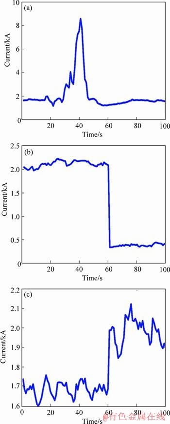
Figure 10 Disturbance of AE in ACS (a) and AC in ACS (b, c)

Table 6 Accuracy in classification with MSD, HULM, SEMTS, EFEST method on XGBoost classifiers to ACS datasets

SEMTS makes an assumption that individual dimensions are independent. Therefore, SEMTS provides one tree for each of the dimensions. After classifying each dimension by shapelet tree, SEMTS chooses the highest accuracy as the final accuracy. It performs badly in datasets whose dimensions are relative to each other. For ACS dataset, if we want to discovery tree in each dimension, information gain is used to measure the goodness of a candidate shapelet. The candidate shapelets are chosen from all samples in each dimension. As shown in Figure 9, the key feature which can distinguish well is not restricted to dimension. If we assess candidate shapelet in one dimension, the key feature will have low information gain. In other words, the key feature can’t be identified by information gain. As a result, we can’t extract the key feature from candidate shapelet. In our method, we assess the candidate shapelet in all dimensions. Therefore, the key feature will be well extracted. Comparing with HULM, the advantage of our method is that it has better interpretability. Shapelets extracted from our method are comprehensible and can offer insight into the problem domain.

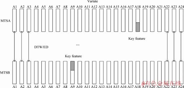
Figure 11 An example of two ACS in same class AC

In Section 3.4, a novel feature of similarity numbers is added to training data. In this section, Table 7 presents the accuracies of XGBoost, k-Neighbor and Gaussian on transformed data which is added feature of similarity numbers. For classifier k-Neighbor and Gaussian, adding feature has little influence on accuracy. However, for classifier XGBoost, adding feature of similarity number presents the best accuracy in 93% of ACS datasets. In Section 4.1.2, we conclude that adding feature of similarity numbers is not always valid for increasing accuracy for every data. If the number of key feature has little influence on class, it’s invalid. In this section, we can conclude that classifier XGBoost performs better accuracy with adding feature. To conclusion, adding feature combining with XGBoost classifier will increase the accuracy of data whose key features’ number influence classifying.

Table 7 Testing accuracy of complex classifiers

Adding feature in XGBoost classifier for ACS datasets can increase accuracy, and the reasons are described as follows. Firstly, key feature can’t identify the time series with one key feature and time series with multi key features for ACS with class AE. The number of time series which are similar to key feature as a new feature can enhance reliability of EFEST algorithm. Secondly, the classifier of XGBoost can ignore the influence of the dominant role of big wave signal to small wave signal. For instance, when the value of feature of similarity numbers is bigger than the one of distance, the feature of similarity numbers will dominate the result of classification. Therefore, XGBoost classifier will increase accuracy for adding feature method.

Lately, we compare the running time of EFEST and MSD in extracting features. For ACS datasets, MSD method takes 22508 s to generate candidate shapelets. However, our method takes 11462 s to generate distance matrix. The results basically confirm our assumption of reducing running time on half. ACS datasets have 24 samples and 24 dimensions. The length of time series in ACS and shapelets are 100 and 30, respectively. Therefore, ACS are big datasets with 40896 candidate shapelets. The more the candidate shapelets, the more the time is taken to calculate than duplicate distance between candidate shapelets. Therefore, the experiment shows the advantage of distance matrix in reducing running time. In Section 4.1.2, we test running time of extracted feature in MSD method and our method. The test results show a bad performance on common datasets in small size. In this section, we prove that distance matrix can reduce complexity of calculation in big datasets.

5 Conclusions and future work

In this work, a concept of MTS with dynamic discriminative subsequence was proposed. We extracted new features with extended shapelet transformation method to classify this kind of MTS. Firstly, key features in one class for all dimension were extracted. Secondly, to increase the reliability of our algorithm, a feature of similarity numbers was added to transformed data. Thirdly, distance matrix was used to extract shapelets and cluster to reduce complexity of calculating. Based on the proposed approach, the influence of dimension on classifying MTS was eliminated.

In order to evaluate the proposed approaches, we gave experimental analyses using 7 common datasets and the ACS datasets. MSD, HULM and SEMTS methods were used to compare with our method. The results of experiment demonstrated that our method had a better performance than other three methods, and our method not only was adaptive to ACS datasets, but also performed well in common datasets. In addition, we pointed out the necessity of distance matrix and adding feature of similarity numbers. Distance matrix reduced the running time for big data. Adding feature of similarity numbers increased the accuracy of our method. The proposed method had a potential application in the local cell condition analysis in the aluminum reduction process. Moreover, this method provided support for intelligent production of aluminum reduction.

In the future, the influence of anode location on extracting key feature in ACS datasets will be taken into consideration. Moreover, the proposed method will be applied to fault location, fault diagnosis and prediction of signal trend.

References

[1] HE Guo-liang, DUAN Yong, PENG Rong, JING Xiao-yuan, QIAN Tie-yun, WANG Ling-ling. Early classification on multivariate time series [J]. Neurocomputing, 2015, 149: 777-787.

[2] KONG Ling-shuang, YANG Chun-hua, LI Jian-qi, WANG Ya-lin. Generic reconstruction technology based on rst for multivariate time series of complex process industries [J]. Journal of Central South University, 2012, 19(5): 1311-1316.

[3] ZENG Ming, LI Jing-hai, MENG Qing-hao, ZHANG Xiao-nei. Temporal-spatial cross-correlation analysis of non-stationary near-surface wind speed time series [J]. Journal of Central South University, 2017, 24(3): 692-698.

[4] MAHARAJ E A, ALONSO A M. Discriminant analysis of multivariate time series: Application to diagnosis based on ecg signals [J]. Computational Statistics & Data Analysis, 2014, 70: 67-87.

[5] MONBET V, AILLIOT P. Sparse vector Markov switching autoregressive models. Application to multivariate time series of temperature [J]. Computational Statistics & Data Analysis, 2017: S0167947316302584.

[6] GORECKI T, LUCZAK M. Multivariate time series classification with parametric derivative dynamic time warping [J]. Expert Systems with Applications, 2015, 42(5): 2305-2312.

[7] ELBAUM S, MALISHEVSKY A G, ROTHERMEL G. Test case prioritization: A family of empirical studies [J]. IEEE transactions on software engineering, 2002, 28(2): 159-182.

[8] YE L, KEOGH E J. Time series shapelets: A new primitive for data mining [C]// Proceedings of the 15th ACM SIGKDD International Conference on Knowledge Discovery and Data Mining. Paris, France, 2009.

[9] ESMAEL B, ARNAOUT A, FRUHWIRTH R K, THONHAUSER G. Multivariate time series classification by combining trend-based and value-based approximations [C]// International Conference on Computational Science and its Applications. Springer, 2012: 392-403.

[10] WENG Xiao-qing, SHEN Jun-yi. Classification of multivariate time series using two-dimensional singular value decomposition [J]. Knowledge-Based Systems, 2008, 21(7): 535-539.

[11] WANG Lin, WANG Zhi-gang, LIU Shan. An effective multivariate time series classification approach using echo state network and adaptive differential evolution algorithm [J]. Expert Systems with Applications, 2016, 43: 237-249.

[12] GHALWASH M F, OBRADOVIC Z. Early classification of multivariate temporal observations by extraction of interpretable shapelets [J]. BMC Bioinformatics, 2012, 13(1):195.

[13] ZHANG Da-hai, QIAN Li-yang, MAO Bai-jin, HUANG Can, SI Yu-lin. A data-driven design for fault detection of wind turbines using random forests and XGboost [J]. IEEE Access, 2018, 6: 21020-21031.

[14] PENG Man-man, LUO Jun. A novel key-points based shapelets transform for time series classification [C]// 2017 13th International Conference on Natural Computation, Fuzzy Systems and Knowledge Discovery (ICNC-FSKD). IEEE, 2017: 2268-2273.

[15] YE L, KEOGH E. Time series shapelets: A novel technique that allows accurate, interpretable and fast classification [J]. Data Mining and Knowledge Discovery, 2011, 22(1,2): 149-182.

[16] FU T C. A review on time series data mining [J]. Engineering Applications of Artificial Intelligence, 2011, 24(1): 164-181.

[17] MUEEN A, KEOGH E, YOUNG N E. Logical-shapelets: An expressive primitive for time series classification [C]// Proceedings of ACM SIGKDD: International Conference on Knowledge Discovery and Data Mining. 2011:

[18] RAKTHANMANON T, KEOGH E. Fast shapelets: A scalable algorithm for discovering time series shapelets [C]// proceedings of the 2013 SIAM International Conference on Data Mining. SIAM, 2013: 668-676.

[19] XING Z Z, JIAN P, YU P S. Early prediction on time series: A nearest neighbor approach [C]// IJCAI 2009, Proceedings of the 21st International Joint Conference on Artificial Intelligence. Pasadena, California, USA, July 11-17, 2009.

[20] PATRI O P, PANANGADAN A V, CHELMIS C, PRASANNA V K. Extracting discriminative features for event-based electricity disaggregation [C]// 2014 IEEE Conference on Technologies for Sustainability (SusTech). IEEE, 2014: 232-238.

[21] HILLS J, LINES J, BARANAUSKAS E, MAPP J, BAGNALL A. Classification of time series by shapelet transformation [J]. Data Mining and Knowledge Discovery, 2014, 28(4): 851-881.

[22] BOSTROM A, BAGNALL A. A shapelet transform for multivariate time series classification [J]. arXiv:1712.06428, 2017.

[23] PATRI O P, KANNAN R, PANANGADAN A V, PRASANNA V K. Multivariate time series classification using inter-leaved shapelets [C]// NIPS 2015 Time Series Workshop. 2015:

[24] GHALWASH M F, RADOSAVLJEVIC V, OBRADOVIC Z. Extraction of interpretable multivariate patterns for early diagnostics [C]// 2013 IEEE 13th International Conference on Data Mining. IEEE, 2013: 201-210.

[25] PATRI O P, SHARMA A B, CHEN H, JIANG G, PANANGADAN A V, PRASANNA V K. Extracting discriminative shapelets from heterogeneous sensor data [C]// 2014 IEEE International Conference on Big Data (Big Data). IEEE, 2014: 1095-1104.

[26] LINES J, DAVIS L M, HILLS J, BAGNALL A. A shapelet transform for time series classification [C]// Proceedings of the 18th ACM SIGKDD International Conference on Knowledge Discovery and Data Mining. ACM, 2012: 289-297.

[27] ZALEWSKI W, SILVA F, MALETZKE A G, FERRERO C A. Exploring shapelet transformation for time series classification in decision trees [J]. Knowledge-Based Systems, 2016, 112: 80-91.

[28] ZHANG Zhen-guo, ZHANG Hai-wei, WEN Yan-long, ZHANG Ying, YUAN Xiao-jie. Discriminative extraction of features from time series [J]. Neurocomputing, 2018, 275: 2317-2328.

[29] PEI W, DIBEKLIOGLU H, TAX D M, van DER MAATEN L. Time series classification using the hidden-unit logistic model [J]. arXiv:1506.05085, 2015.

[30] CETIN M S, MUEEN A, CALHOUN V D. Shapelet ensemble for multi-dimensional time series [C]// Proceedings of the 2015 SIAM International Conference on Data Mining. SIAM, 2015: 307-315.

[31] RISH I. An empirical study of the naive Bayes classifier [C]// IJCAI 2001 Workshop on Empirical Methods in Artificial Intelligence. Seattle, Washington, USA: IJCAI, 2001: 41-46.

[32] YUE Wei-chao, CHEN Xiao-fang, GUI Wei-hua, XIE Yong-fang, ZHANG Hong-liang. A knowledge reasoning fuzzy-Bayesian network for root cause analysis of abnormal aluminum electrolysis cell condition [J]. Frontiers of Chemical Science and Engineering, 2017, 11(3): 414-428.

[33] EICK I, KLAVENESS A, ROSENKILDE C, SEGATZ M, GUDBRANDSEN H, SOLHEIM A, SKYBAKMOEN E, EINARSRUD K. Voltage and bubble release behaviour in a laboratory cell at low anode-cathode distance [C]// Proc. 10th Australasian Aluminium Smelting Technology Conference, Launceston, TAS. 2011.

[34] CHEUNG C-Y, MENICTAS C, BAO J, SKYLLAS-KAZACOS M, WELCH B J. Characterization of individual anode current signals in aluminum reduction cells [J]. Industrial & Engineering Chemistry Research, 2013, 52(28): 9632-9644.

[35] YANG Shuai, ZOU Zhong, LI Jie, ZHANG Hong-liang. Online anode current signal in aluminum reduction cells: Measurements and prospects [J]. JOM, 2016, 68(2): 623-634.

(Edited by ZHENG Yu-tong)

中文导读

一种基于动态鉴别性序列的多变量时间序列分类方法及在阳极电流信号上的应用

摘要：多变量时间序列的分类方法是时间序列知识发现的重要组成部分。因此，提出了多种多变量时间序列分类方法。然而，大部分的多变量时间序列方法都没有考虑鉴别性特征不受维度限制的时间序列。因此，本文提出了一种基于shapelet转换的特征提取方法。首先，从同一类别中的所有维度的候选shapelet中提取核心特征，它代替k个shapelet计算距离。其次，利用相似数量特征去加强分类的可靠性。最后，为缩短搜索和聚类shapelet的时间使用了距离矩阵。基于公共数据集的实验结果表明了该方法的有效性，且将实验结果成功地应用于阳极电流信号的分类。

关键词：阳极电流信号；核心特征；距离矩阵；相似数量特征；shapelet转换

Foundation item: Projects(61773405, 61725306, 61533020) supported by the National Natural Science Foundation of China; Project(2018zzts583) supported by the Fundamental Research Funds for the Central Universities, China

Received date: 2019-01-06; Accepted date: 2019-08-30

Corresponding author: CHEN Xiao-fang, PhD, Professor; Tel: +86-13787276890; E-mail: xiaofangchen@csu.edu.cn; ORCID: 0000- 0002-7188-032X