Dynamic phase-mining optimization in open-pit metal mines

GU Xiao-wei(顾晓薇), WANG Qing(王 青), GE Shu(葛 舒)

College of Resource and Civil Engineering, Northeastern University, Shenyang 110004, China

Received 12 July 2009; accepted 11 September 2010

Abstract: Three important aspects of phase-mining must be optimized: the number of phases, the geometry and location of each phase-pit (including the ultimate pit), and the ore and waste quantities to be mined in each phase. A model is presented, in which a sequence of geologically optimum pits is first generated and then dynamically evaluated to simultaneously optimize the above three aspects, with the objective of maximizing the overall net present value. In this model, the dynamic nature of the problem is fully taken into account with respect to both time and space, and is robust in accommodating different pit wall slopes and different bench heights. The model is applied to a large deposit consisting of 2 044 224 blocks and proved to be both efficient and practical.

Key words: open-pit; phase-mining; dynamic programming; optimization

1 Introduction

Phase-mining (also referred to as stage-mining) is widely practiced in large open-pit mines or relatively small ones where topographies and ore-body geometries are suitable. Three important aspects of phase-mining must be optimized to maximize the overall net present value (NPV): the number of phases, the geometry and location of each phase-pit (including the ultimate pit), and the ore and waste quantities to be mined in each phase. Therefore, planning a phase-mining operation is a combination of pit designing and production scheduling.

Pit optimization, when seen as an isolated problem, may be considered a solved problem. The optimization algorithm by LERCHS and GROSSMANN[1] has been regarded as the landmark in this field. It has been implemented in a number of commercial software packages such as Whittle, MapTek and DataMine. Recent research on the pit optimization problem has been largely based on incorporation of various relevant parameters and/or conditions and different approaches have been proposed. FRIMPONG et al[2] incorporated structural, hydrological, and geotechnical conditions in the ultimate pit design problem and used neural network and artificial intelligence for solution. JALALI et al[3] considered uncertainties of different pit geometries and used Markevian chains to determine the ultimate pit.

The production scheduling problem is much more complicated and research activities are still going on. Almost all models/algorithms for production schedule optimization are based on regular block models with the objective of determining the best sequence of mining the blocks so that the NPV is maximized. One of the major difficulties lies in the formidable size of the problem. The block model for a real life deposit can easily contain hundreds of thousands to millions of blocks. Therefore, substantial efforts have been focused on reducing the size of the problem or devising heuristic algorithms to enhance the efficiency and applicability of the solution process[4].

A common way of reducing the size of the production scheduling problem is to first combine blocks into block aggregates and then take the aggregates as decision units in various sequencing schemes. SAMANTA et al[5] aggregated blocks into layers and employed a genetic algorithm to heuristically solve the sequencing problem. KAWAHATA[6] used reserve parameterization (a more sophisticated way of aggregation) and Lagrangian relaxation procedure to solve the problem. HALATCHEV[7] proposed a bench-sequencing approach, in which benches were generated in the ultimate pit and then sequenced based on specified rules. RAMAZAN[8] developed another way of block aggregation by constructing “fundamental trees” through linear programming.

Various heuristic algorithms were developed to facilitate the solution of the production scheduling problem. CACCETTA and HILL[9] used a branch- and-cut approach, in which breadth-first search and depth-first search were considered to get possible schedules and implemented a linear programming based heuristic algorithm. BLEY et al[10] formulated an integer programming model and used a variable reduction technique by combining the production constraints and the precedence constraints among the blocks to form a so-called precedence-constrained knapsack for each time period and each attribute. BOLAND et al[11] used binary variables to enforce precedence between aggregates of blocks and continuous variables to control the amount of material extracted from each of the aggregates and from each block within an aggregate. AMAYA et al[12] developed a random, local search heuristic algorithm that seeks to improve on an incumbent integer programming solution by iteratively fixing and relaxing part of the solution. GHOLAMMEJAD and OSANLOO[13] considered block-grade uncertainty in their model, with each block having a probability distribution function obtained through geostatistical simulation. A genetic algorithm was used to solve the problem.

For phase-mining, independently optimizing one phase at a time will not maximize the overall NPV due to the dynamic interactions among the phases. In this work, a dynamic phase-mining optimization model is presented, in which the interactions are fully accounted for. The basic idea was first proposed by WANG and SEVIM[14-15] in their production planning model. Improvements have been made to make it suitable to phase-mining optimization and also more efficient, optimal and practical.

2 Generation of geologically optimum pits

A “geologically optimum” pit for a given total tonnage (ore plus waste), T, is the pit that contains the maximum metal quantity of all the pits of the same total tonnage.

It is not hard to imagine that there exist numerous, theoretically an infinite number of, pits for any given total tonnage, having different shapes and/or locations. Finding the one with the maximum metal quantity entails an efficient search in the block model. The objective is to obtain a sequence of nested geologically optimum pits with a desired increment, ΔT, between two adjacent pits. The basic idea is that finding the geologically optimum pit of total tonnage, T, is equivalent to eliminating the least-metal portion, ΔT, from a larger geologically optimum pit of total tonnage, T+ΔT. Based on this idea, the process of generating a sequence of geologically optimum pits starts with the largest possible pit for the deposit.

The largest possible pit for the deposit is obtained in two steps. In the first step, a geometric bounding is used to obtain a pit so that its limit on the ground surface is the same as the property boundary. In the second step, a big enough instantaneous strip ratio, R_S (net loss will definitely occur at this strip ratio), is used to further bound the pit, by eliminating those portions at the pit walls and pit bottom whose strip ratios are equal to or greater than R_S. The detailed algorithms for pit bounding will not be presented here. The result of the geometric and strip-ratio bounding is the largest possible pit, which is also the largest geologically optimum pit, denoted   as P_n.

The algorithm is hereafter explained on a 2D cross section without losing generality. Suppose a cross section of this largest pit, P_n, as shown in Fig.1. The blocks are shown as grids whose heights are equal to the corresponding bench heights, and different bench heights can be used for different benches. The bottom elevation of each vertical block column is at the pit wall or pit bottom at the column center, and the top elevation at the ground surface. For accurate calculation of ore and waste quantities and for accurate compliance to the given pit wall slopes, a block column within the pit may not have an integer number of bocks. Partial blocks are used at the pit walls, ground surface and pit bottoms, if necessary.

Fig.1 Illustration of pit and cone evaluated for possible elimination

First, a cone template is constructed, whose surface angles with respect to the horizontal plane are equal to the pit wall slopes in pre-specified directions. If the pit wall has different slopes in different zones, a cone template is constructed for each zone.

Then, the cone apex is placed at the center of the lowest block of a column (i.e. the lowest block of the column whose center falls inside P_n). The cone whose apex is at the center of the lowest block of column 5 is depicted in Fig.1. The metal quantity, total tonnage, and the metal content per ton of the cone within the pit are calculated based on the grades of the whole and partial blocks that fall below the cone surface and above the pit (blocks in the dot-shaded narrow area). The cone location and its metal content per ton are stored in an array. After the cone apex is moved and placed at the centers of the lowest blocks of all the columns and the same calculations are done after each movement, an array of all the cone locations and their associated metal contents per ton is obtained. To save computer memory and execution time, those cones with total tonnages greater than the specified pit increment, ΔT, are discarded. This process is hereafter referred to as “a round of scanning”.

The array elements, with each recording the location and metal content per ton of a cone, are then sorted in an ascending order with respect to their metal contents per ton, so that the first element has the least metal content per ton and the last the most. Suppose that there are N elements in the array. A union of the first M cones corresponding to the first M elements is sought, such that the total tonnage of the union, denoted by T_u, is equal to or smaller than the pit increment, ΔT. The blocks in the union of these M cones are eliminated from pit P_n by raising the bottom elevation of each column affected by one or more of the M cones to the corresponding cone surface. A new pit is thus obtained whose total tonnage is T_u tons smaller than P_n.

If T_u is equal to or close enough to the pit increment, ΔT, the new pit is the next smaller geologically optimum pit, whose total tonnage is ΔT (or sufficiently close to ΔT) tons smaller than that of P_n.

If T_u is smaller than and not sufficiently close to the pit increment, ΔT, another round of scanning is done based on the new pit and a union of least-metal content cones is sought, so that its total tonnage in the new pit is equal to or smaller than ΔT-T_u. The blocks in the cone union are eliminated. This process of scanning and eliminating continues until ΔT (or sufficiently close to ΔT) tons are eliminated from pit P_n, resulting in the next smaller geologically optimum pit, denoted as P_n-1.

Based on P_n-1 and repeating the above process, the next smaller pit, P_n-2, can be obtained, and then the next smaller pit, P_n-3 based on P_n-2, until the tonnage of the remaining portion is equal to or smaller than the desired tonnage of the smallest pit P₁. A sequence of geologically optimum pits is obtained.

Since in each round of scanning, the portion that contains least metal content per ton is eliminated, the remaining pit after the elimination has the maximum (or very close to the maximum) metal quantity of all pits with the same total tonnage. Therefore, each of the pits thus generated is geologically optimum (or very close to the optimum). Also, since the surface slopes of the cone are the same as the pit wall slopes in pre-specified directions/zones and partial blocks are used at the pit walls, the resulting pit after each round of scanning and eliminating does not violate slope constraints. Furthermore, since each pit is generated based on a larger pit, the pits are nested.

3 Dynamic optimization model

Once a sequence of n geologically optimum pits, {P₁, P₂, …, P_n-1, P_n}, is generated with a small enough increment, ΔT, and sorted from the smallest to the largest, these pits are the best candidates for each of the phase-pits to be designed. They are the best candidates because, if it is decided to mine T tons of total material at the end of a phase, mining the geologically optimum pit corresponding to T is certainly better than mining any other pits of the same total tonnage. Therefore, the problem of determining the best phase-pits becomes a problem of determining which pit in the geologically optimum pit sequence should be used as the phase-pit for that phase, so that the overall NPV is maximized.

The n geologically optimum pits are placed in a dynamic programming scheme shown in Fig.2. The horizontal axis represents stage and the vertical axis state. The states of a stage correspond to the geologically optimum pits arranged from the smallest to the largest. The number of stages is equal to the number of geologically optimum pits, n. An arrow represents a transition from a state of a stage to a state of the next stage. For the purpose of clarity, not all transitions are drawn in Fig.2. Since any pit of stage i is expanded (through mining) from a smaller pit of the preceding stage i-1, a state transition can only go upwards to a pit of current stage from smaller pits of the preceding stage. This is why the starting state of stage i (the lowest state) corresponds to pit P_i (i = 1, 2, …, n).

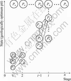
Fig.2 Stages and states in dynamic programming formulation

In general, considering state j of stage i, the pit associated with this state is P_j and can be transited from those states of the preceding stage, i-1, whose corresponding pits are smaller than P_j, as shown in Fig.2. When pit P_j of stage i is transited from pit P_k (i-1 ≤ k ≤ j-1) of stage i-1, the metal quantity m_{i, j}(i-1, k), ore quantity q_{i, j}(i-1, k), and waste quantity w_{i, j}(i-1, k) mined for such a transition are

m_{i, j}(i-1, k) = M_j-M_k                                         (1)

q_{i, j}(i-1, k) = Q_j-Q_k                           (2)

w_{i, j}(i-1, k)= W_j-W_k                                          (3)

where M_j and M_k are the metal quantities contained in pits P_j and P_k, respectively; Q_j and Q_k are the ore quantities contained in pits P_j and P_k, respectively; W_j and W_k are the waste quantities contained in pits P_j and P_k, respectively.

Assume that the final product of the mining enterprise is ore concentrate. A simplified calculation of the profit, P_i,j(i-1, k), made for such a transition is given by

    (4)

where R_m and R_p are the recovery rates of mining and ore processing, respectively; G_p is the grade of concentrate, p_i is the price of ore concentrate in stage i, which could be a constant; Y is the waste-mixing rate of mining; C_m, C_p, and C_w are the unit costs of ore mining, processing, and waste removing, respectively.

Supposing that the ore mining capacity, waste removing capacity, and the ore processing capacity have a perfect match, the time length, t_i,j(i-1, k), required to make such a transition, i.e. to mine q_i,j(i-1, k) quantity of ore, is

              (5)

where m_i is the yearly ore mining capacity. If the capacities do not match, the longest time of ore mining, waste removing, and ore processing should be used.

t_{i, j}(i-1, k) may not be an integer number of years. Let L_{i, j}(i-1, k) be the integer part and δ_{i, j}(i-1, k) be the decimal part of t_i,j(i-1, k), respectively. The average annual profit for each of the L_{i, j}(i-1, k) years is denoted by a_{i, j}(i-1, k) and is equal to

                         (6)

The remaining profit for the decimal part, δ_i,j(i-1, k), is denoted by r _i,j(i-1, k) and is

 (7)

The cumulative time to arrive at pit P_j of stage i, denoted by T_i,j(i-1, k), when it is transited from pit P_k of stage i-1, is

T_{i, j}(i-1, k)=T_{i-1, k}+t_{i, j}(i-1, k)                    (8)

where T_{i-1, k} is the cumulative time to arrive at pit P_k of stage i-1, following the best route (policy) in the network shown in Fig.2.

Hence, the cumulative NPV realized at pit P_j of stage i, denoted by V_{i, j}(i-1, k), when it is transited from pit P_k of stage i-1, is given by

  (9)

where V_{i-1, k} is the cumulative NPV associated with pit P_k of stage i-1, when arrived following the best route; d is the discount rate.

It is clear from Fig.2 that pit P_j of stage i may be transited from different pits of the preceding stage i-1. Obviously, when pit P_j of stage i is transited from a different pit of stage i-1, the metal quantity, ore quantity, and waste quantity mined in the transition (Eqs.(1)-(3)) will be different, and the time length and profit will be different, too. Consequently, the cumulative NPV at pit P_j of stage i varies with different transitions (decisions). The transition with the highest cumulative NPV is the best transition (optimum decision) and, thus, the recursive function is

                   (10)

The initial conditions at time 0 are

                                  (11)

Using the above equations and starting from the first stage, the pits (states) are evaluated forward stage by stage, until all the pits of all stages in Fig.2 are evaluated. The best transitions and associated cumulative NPVs are obtained for all the pits of all stages. Then, the pit that has the highest cumulative NPV of all pits of all stages is found. This pit is the best ultimate pit, and the stage at which it is found indicates the best number of phases. For example, supposing that the number of geologically optimum pits is 20, the number of stages in the dynamic programming scheme is also 20. If the pit with the highest cumulative NPV is found at stage 4, and this pit is the 11th pit, P_11, in the pit sequence, the deposit should be mined in 4 phases and the best ultimate pit is P₁₁.

Starting from the best ultimate pit and tracing the best transitions backward to the first stage, the optimum route can be found, which is called the optimum policy in dynamic programming. This optimum policy simultaneously indicates the number of phases (as discussed above), the geometry and location of each phase-pit (including the ultimate pit), and the ore quantity and waste quantity to be mined in each phase.

4 Application

A software package was developed based on the model and was applied to a large open-pit mine (which is not named here for confidentiality of data). The mine has been in operation for many years and its future phases are being designed. The current topography of the mine is shown in Fig.3. The block model of the deposit contains 2 044 224 blocks whose size on the horizontal plane is 25 m × 25 m with a height equal to the bench height. The bench height is 12 m above the 238 m level and 15 m below. A cross section of the block model is shown in Fig.4 where the shaded blocks are ore blocks. Seven different final slope angles were used for seven sectors, ranging from 34.5° to 51.0°. The economic and technical parameters are listed in Table 1.

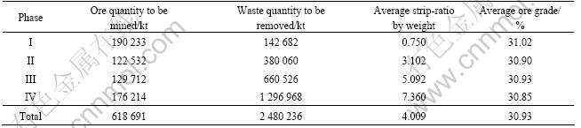
The mining phases were optimized based on the above information. The best number of phases in the optimum solution is 4 and the four phase-pits are shown in Fig.5. A cross section of the four phase-pits superimposed on the cross section of the block model is shown in Fig.6. The best ore and waste quantities to be mined in each of the four phases are listed in Table 2.

It can be seen that with an annual ore production rate of 15×10⁶, the time span of the phases ranges from 8.2 to 12.7 years with a total mine life of a little over 41 years. The time spans of the phases are reasonable because most of the expensive heavy equipment used in open-pit mining (e.g. shovels, drills, trucks) has an economical service life within the above range.

The optimum solution may not be feasible at some

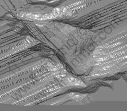
Fig.3 Perspective 3-D view of current topography of mine

Fig.4 Cross section of block model of deposit

locations from a practical point of view because it is not possible to incorporate all practical constraints in a mathematical model. In Fig.6, for example, the horizontal distance between the phase II pit and the phase III pit on the right-hand side is less than 30 m, obviously too narrow to be practical on this cross section. In such cases, manual adjustment of the phase-pit contours is needed to arrive at a feasible solution.

The optimum solution to the phase-mining problem for a given deposit depends on the parameters listed in Table 1. Sensitivity analyses with respect to any of these parameters can be easily done by using the developed software. Such analyses are valuable in arriving at the final decision.

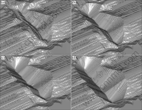
Fig.5 Perspective 3D view of best phase-pits: (a) Phase I pit; (b) Phase II pit; (c) Phase III pit; (d) Phase IV pit (Ultimate pit)

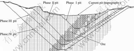
Fig.6 Best phase-pits on cross section of block model

Table 2 Ore and waste tonnages and ore grades mined in each phase

5 Conclusions

1) The dynamic nature of the phase-mining optimization problem with respect to both time and space is fully accounted.

2) Simultaneous solutions can be obtained: the number of phases, the geometry and location of each phase-pit (including the ultimate pit), and the ore and waste quantities to be mined in each phase.

3) The pit-generation algorithm is robust in which different pit wall slopes can be specified in pre-defined directions or zones and the resulting phase pits have nearly perfect compliance to the pit wall slopes, and different bench heights can also be used.

4) Application of the model demonstrated that it is computationally efficient and is quite capable of handling large deposit models containing above a million blocks.

References

[1] LERCHS H, GROSSMANN I. Optimum design of open-pit mines [J]. Canadian Institute of Mining, Metallurgy and Petroleum Bulletin, 1965, 58(1): 17-24.

[2] FRIMPONG S, ASA E, SZYMANSKI J. Intelligent modeling: Advances in open pit mine design and optimization research [J]. International Journal of Surface Mining, Reclamation and Environment, 2002, 16(2): 134-143.

[3] JALALI S E, ATAEE-POUR M, SHAHRIAR K. Pit limits optimization using a stochastic process [J]. Canadian Institute of Mining Magazine, 2006, 1(6): 90-94.

[4] NEWMAN A M, RUBIO E, WEINTRAUS A, CARO R, EUREK K. A review of operations research in mine planning [EB/OL]. Articles in advance, Informs, http//interfaces.journal. informs.org/cgi/reprint/inte.1090.0492v1.

[5] SAMANTA B, BHATTACHERJEE A, GANGULI R. A genetic algorithms approach for grade control planning in a bauxite deposit [C]//GANGULI R, DESSUREAULT S, KECOJEVIC V, DWYER J. Proceedings of the 32nd International Symposium on Applications of Computers and Operations Research in the Mineral Industry. Littleton, USA: SME, 2005: 337-342.

[6] KAWAHATA K. A new algorithm to solve large scale mine production scheduling problems by using the Lagrangian relaxation method [D]. Golden, USA: Colorado School of Mines, 2006: 1-217.

[7] HALATCHEV R. A model of discounted profit variation of open pit production sequencing optimization [C]//GANGULI R, DESSUREAULT S, KECOJEVIC V, DWYER J. Proceedings of the 32nd International Symposium on Applications of Computers and Operations Research in the Mineral Industry. Littleton, USA: SME, 2005: 315-323.

[8] RAMAZAN S. The new fundamental tree algorithm for production scheduling of open pit mines [J]. European Journal of Operations Research, 2007, 177(2): 1153-1166.

[9] CACCETTA L S, HILL P. An application of branch and cut to open pit mine scheduling [J]. Journal of Global Optimization, 2003, 27(2): 349-365.

[10] BLEY A, BOLAND N, FRICKE C, FROYLAND G. A strengthened formulation and cutting planes for the open pit mine production scheduling problem [J]. Computers & Operations Research, 2010, 37(9): 1641-1647.

[11] BOLAND N, DUMITRESCU I, FROYLAND G, GLEIXNER A M. LP-based disaggregation approaches to solving the open pit mining production scheduling problem with block processing selectivity [J]. Computers & Operations Research, 2009, 36(4): 1064-1089.

[12] AMAYA J, ESPINOZA D, GOYCOOLEA M, MORENO E, PREVOST T, RUBIO E. A scalable approach to optimal block scheduling [C]//Proceedings of the 35th International Symposium on Applications of Computers and Operations Research in the Mineral Industry. Vancouver, Canada: CIM, 2010: 567-571.

[13] GHOLAMMEJAD J, OSANLOO M. Using chance constrained binary integer programming in optimizing long term production scheduling for open pit mine design [J]. Transactions of the Institution of Mining and Metallurgy, Section A, 2007, 116(2): 58-66.

[14] WANG Q, SEVIM H. Open pit production planning through pit-generation and pit-sequencing [J]. Transactions of the American Society for Mining, Metallurgy and Exploration, 1993, 294(7): 1968-1972.

[15] WANG Q, SEVIM H. Alternative to parameterization in finding a series of maximum-metal pits for production planning [J]. Mining Engineering, 1995(2): 178-182.

(Edited by YANG Bing)

Foundation item: Project(50974041) supported by the National Natural Science Foundation of China; Project(20090042120040) supported by the Doctoral Program Foundation of the Ministry of Education, China; Project(20093910) supported by the Natural Science Foundation of Liaoning Province, China

Corresponding author: WANG Qing; Tel: +86-24-83678400; Fax: +86-24-83680388; Email: qingwangedu@163.com

DOI: 10.1016/S1003-6326(09)60404-0