Trans. Nonferrous Met. Soc. China 27(2017) 184-196

Dynamic behavior of rock during its post failure stage in SHPB tests

Zi-long ZHOU¹, Yuan ZHAO¹, Yi-hui JIANG², Yang ZOU³, Xin CAI¹, Di-yuan LI¹

1. School of Resources and Safety Engineering, Central South University, Changsha 410083, China;

2. China Railway Engineering Consulting Group Co., Ltd., Beijing 100000, China;

3.  Polytechnique  de Lausanne (EPFL), School of Architecture, Civil and Environmental Engineering, Lausanne CH-1015, Switzerland

Received 20 November 2015; accepted 9 October 2016

Abstract: In order to investigate the micro-process and inner mechanism of rock failure under impact loading, the laboratory tests were carried out on an improved split Hopkinson pressure bar (SHPB) system with synchronized measurement devices including a high-speed camera and a dynamic strain meter. The experimental results show that the specimens were in the state of good stress equilibrium during the post failure stage even when visible cracks were forming in the specimens. Rock specimens broke into strips but still could bear the external stress and keep force balance. Meanwhile, numerical tests with particle flow code (PFC) revealed that the failure process of rocks can be described by the evolution of micro-fractures. Shear cracks emerged firstly and stopped developing when the external stress was not high enough. Tensile cracks, however, emerged when the rock specimen reached its peak strength and played an important role in controlling the ultimate failure during the post failure stage.

Key words: rock dynamics; post failure; stress equilibrium; crack evolution; particle flow code

1 Introduction

The post failure refers to the material’s deformation after its peak strength. The post failure behavior is essential for understanding the rupture process of rock materials. Especially, as cracks come forth and evolve after peak strength, the rock specimen at its post failure stage is a close analogy to engineering rock masses full of micro-cracks or joints. The post failure behavior can give crucial information about the mechanism of many engineering hazards such as rock-burst and large scale collapse of rock masses [1,2]. However, sudden failure of rock materials makes it very difficult to determine the post failure properties in practice.

In static tests, an effective method has been built to get the post failure behavior of rocks. Researches in 1960s first found that rock specimens usually collapse violently soon after reaching the ultimate strength when a normal hydraulic ram machine was used [3-6]. It is recognized that this kind of machines were too compliant. Once the specimen started to lose its load- carrying ability, the loading system released more energy than that could be absorbed by the slow deformation of the specimen. The excess energy caused the specimen to fail violently [1]. BARNARD [3] designed a system involving minimum fluid volume which successfully got the post peak stress-strain curve of concrete. WAWERSIK et al [4,5] and HUDSON et al [6] successfully applied a rapid-unloading technique to experimental equipment which could make the breakdown process of rock controllable.

Study of rock dynamics has a short history, and lots of problems still remain unsolved [7]. To get the dynamic behavior of materials, gas-driven machines, drop weight, SHPB, Taylor test, plate impact, etc., have been tried in the researches before [8-11]. Although most of them can be used to estimate the dynamic strength approximately, only the SHPB method can record the deformation process of specimens. However, when the traditional SHPB is used for rock materials, the basic assumptions of this technique cannot be well satisfied [12-14]. In recent years, lots of improvements have been made on SHPB device for rock tests. Pressure bar with diameter of 50 mm has been used to accommodate with the rock specimens, whose grain size is bigger than that of metal [13]. Pulse shaping methods have been brought up to generate slowly rising incident waves to overcome premature failure [15,16]. With these efforts, SHPB is now suggested as ISRM test method to determine the dynamic strength and toughness of rocks [17]. However, there are still a few studies about the dynamic failure process of rocks in SHPB tests, even less about the post failure stage. When rocks are subjected to dynamic loadings, they reach their peak strength quickly and fail suddenly, and the failure strain is less than 1%. During the post failure stage, rocks deform even more quickly. The stress equilibrium state becomes even more difficult and crucial for evaluation of the behavior of rock at this stage. Recently, various optical methods, such as high-speed photography, digital image correlation (DIC), virtual field method (VFM), and numerical method have brought possibility to investigate more details of the behavior of rocks at post failure stage [18-22]. ZHANG et al [19] used DIC method for dynamic compression tests and monitored the very small strain in brittle rock materials, however, the limitation of camera’s resolution made it difficult for a direct measurement of the post failure behavior. LI et al [20] simulated the deformation process of rocks in SHPB tests with PFC. In their research, the stress equilibrium, strain rate, heterogeneity effects were investigated, but the experimental results which could be compared with the simulated results were lacking.

In this study, to study the post failure behavior of rock, dynamic tests on granite specimens were carried out on SHPB, and the failure processes were captured by a high-speed camera. The stress equilibrium of specimens under different strain rates were also investigated in detail. Moreover, to further reveal the micro-mechanism of rocks during the post failure stage, numerical simulations with particle flow code (PFC) were conducted and the micro-fracturing process was evaluated from the crack evolution.

2 Experimental

2.1 Rock material and specimen preparation

The rock material used in this study is granite obtained from Fujian Province, China. The mineralogical composition was obtained by means of scanning electron microscope (SEM), as shown in Fig. 1. This granite consists of 64% feldspar, 29% quartz, 2%-5% biotite and the particle size of minerals is from 4 to 50 μm. The density and P-wave velocity of this granite are 2650 kg/m³ and 4860 m/s.

All specimens in this work were extracted from one granite block with high geometrical integrity and petrographic uniformity. Special care was taken in preparing the cylindrical specimens with nominal diameter of 50 mm and height of 50 mm [17]. All specimens were polished to make the surface roughness less than 0.02 mm and the end surface perpendicular to its axis less than 0.001 rad. Before dynamic SHPB tests, standard static compression tests [23] were conducted. The parameters and results of the specimens are listed in Table 1.

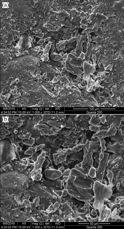
Fig. 1 SEM images of the Fujian granite

2.2 Apparatus of SHPB system

Dynamic compressive tests were conducted using a modified SHPB setup suggested by the ISRM [17]. The setup consists of a cone-shaped striker, an input bar (2.0 m in length), an output bar (2.0 m in length), an absorption bar (0.5 m in length) and other auxiliary components such as a gas gun and a data acquisition unit. The bars and striker are made of high strength 40Cr steel with density of 7800 kg/m³, elastic modulus of 240 GPa and yield strength of about 1000 MPa.

During a test, the striker is driven by the high-pressure gas in the gas gun and impacts the front end of the input bar. Upon impacting, longitudinal stress wave (incident wave) is generated and propagates towards the specimen. In addition, by changing the impact gas pressure in the gas gun, the striker can be shot with different velocities and produces stress waves with different magnitudes, which causes the specimens to deform with different strain rates.

When the incident wave reaches the input bar/specimen interface, part of it is reflected, while the remaining part goes through the specimen and transmits into the output bar. With strain gauges attached on the input and output bars, the incident wave, reflected wave and transmitted wave can be collected. According to the SHPB theories, the stress, strain and strain rate of the specimen can be calculated as follows [17]:

                (1)

                (2)

                    (3)

where A_e, C_e and E_e are the cross-sectional areas, wave velocity, and elastic modulus of elastic bars; A_s and L_s are the cross-sectional area and the length of the specimen;  is the strain rate of the specimen; ε_I, ε_R, and ε_T represent the incident, reflected and transmitted strains, respectively.

During tests, a high-speed camera (FASTCAM SA1.1) was used to record the failure process of specimens. The frame rate was 100000 fps (frames per second), and the exposure time was 10 μs, covering about 192×192 pixels. These settings conditioned upon each other and were selected to obtain the best results for the tests. The automatic trigger of this camera was achieved by a transistor-transistor logic (TTL) level signal, which was generated by the oscilloscope when it was triggered by the incident wave. In this way, the strain signal and the images were recorded synchronously and the relative time of the images with respect to the loading process can be determined.

3 Results and discussion

Table 1 gives the parameters and test results of granite specimens. In each strain rate group, 3 specimens were tested. And only results of the representative specimens (D-1-1, D-2-2, D-3-3) were chosen for analyses in this study. The stress, strain and strain rate were obtained by Eqs. (1)-(3), respectively.

3.1 Deformation characteristic and stress equilibrium of specimens at different strain rates

According to the SHPB principles, dynamic stress equilibrium in the specimen should be satisfied to ensure test results validity [9,14]. To further quantitatively evaluate the stress equilibrium, the stress equilibrium factor was defined as

                          (4)

where σ_I, σ_R and σ_T are the incident, reflected and transmitted stresses corresponding to ε_I, ε_R and ε_T, respectively. When this factor approaches zero, the stress at the two ends of the specimen reaches a perfect force/stress balance state.

Table 1 Parameters and test results of specimens in laboratory tests

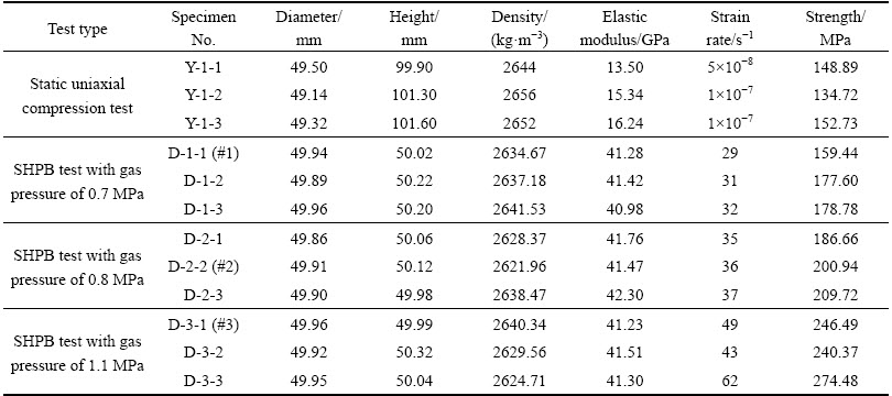
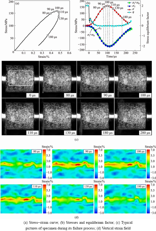
Fig. 2 Experimental results of representative specimen #1

Figure 2 shows the experimental results of the representative specimen #1 (D-1-1) at the strain rate of about 29 s^-1. From Fig. 2(a), it can be seen that, under the impact loading, the specimen began to deform elastically. Since 80 μs, the elastic modulus decreased slightly, which indicated that internal degradation happened. At 100 μs, the inner stress of the specimen reached a maximum of 160 MPa. After that, as the incident stress gets weaker, the external stress could not support the specimen to deform to a higher stress level, the strain increased slightly and then decreased just like the unloading process. Figure 2(b) presents the stress history for specimen D-1-1, it can be observed that, the curve of the sum of the incident and reflected waves almost overlaps with that of the transmitted wave. The stress equilibrium factor indicates that the specimen D-1-1 reached the state of stress equilibrium at about 30 μs, and kept this state till 180 μs.

Figure 3 gives the experimental results of the representative specimen #2 (D-2-2) at the strain rate of about 36 s^-1. Figure 3(a) shows that the specimen also experienced elastic deformation and modulus/stiffness decrease. The specimen reached its peak strength of 200 MPa at 110 μs, which is much bigger than that of the specimen #1 because of the higher magnitude of the incident stress. Figure 3(b) shows that the specimen remained in the state of stress equilibrium from 50 μs to 170 μs.

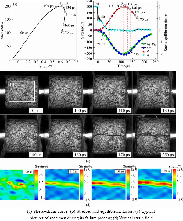
Fig. 3 Experimental results of representative specimen #2

Figure 4 gives the experimental results of the specimen #3 (D-3-1) at the strain rate of about 49 s^-1. It can be seen that the specimen reached its peak strength, 246.49 MPa, at 100 μs. The stress equilibrium of the specimen was well kept between 50 μs and 180 μs.

From Figs. 2-4, it can be concluded that the specimens in SHPB tests can keep in the state of good stress equilibrium at the post failure stage, although cracks may form and spread through it. This indicates that the basic assumption of the SHPB technique can be satisfied and the SHPB device can give accurate results for the post failure stage of rock specimens.

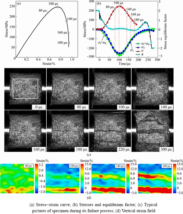
Fig. 4 Experimental results of representative specimen #3

3.2 Failure patterns of specimens at different strain rates

In order to study dynamic failure patterns of specimens, high-speed camera was used to take pictures of the failure process and these pictures were analyzed by digital image correlation (DIC) technique to trace cracks.

Figures 2(c) and (d) show typical pictures of the specimen #1 (D-1-1). At 80 μs, a small crack appeared on the specimen’s surface and grew slightly till 100 μs. When the specimen passed its peak strength around 110 μs, it is found that the crack began to close gradually. At 180 μs, however, the crack became invisible.

The photographical records in Figs. 3(c) and (d) show that the first visible crack emerged at 100 μs on specimen #2 (D-2-2). Then the crack grew rapidly and ran through the specimen at 140 μs. After that, the width of the crack became larger and larger.

Figures 4(c) and (d) show the failure process of specimen #3 (D-3-1). The photographical record reveals that multiple cracks formed along the loading direction. At 160 μs, two cracks became very obvious, and then more cracks appeared. Even in this case, the specimen was still in the state of good stress equilibrium until 180 μs.

The high speed camera could record the transient information of the crack evolution but only the side view of the specimen was provided. After each test, the specimen and its fragments were collected and put together.

Figures 5(a) shows that the specimen #1 stayed intact as a whole. But careful check reveals that there were cracks at both ends and the side of the specimen. The cracks at the ends presented a ring shape around the specimen’s axis. The cracks at the side face propagated along the direction parallel to the specimen’s axis.

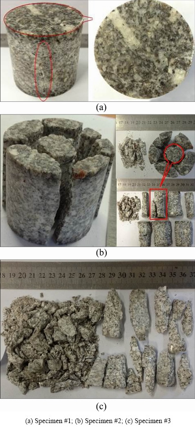
Fig. 5 Failure patterns of specimens at different strain rates

The failure pattern of the specimen #2 (Fig. 5(b)) shows that the specimen broke into slim strips. When putting all the fragments together, the original shape of the specimen could be recovered. And these strips were strong enough to resist the bending force of adult hands.

The specimen #3 was crushed into little pieces as shown in Fig. 5(c). But Fig. 4(c) shows that the specimen #3 was in close contact with steel bar until 180 μs, when the stress was below 30% of peak stress.

Generally, the failure of the specimens is mainly caused by cracks from two groups. One group of cracks emerges from the side of the specimen and spreads along the loading direction. Another group of cracks forms at the contact ends between the steel bar and the specimen. Then cracks of this group connect each other, forming a ring shape. With the increase of the strain rates, the cracks accumulate more intensively in the specimen. Finally, the specimen breaks into slim strips and these strips still have great strength along the loading direction. Thus the specimen still keeps the state of stress equilibrium during its post failure stage.

4 Numerical investigations

Laboratory tests can give intuitive knowledge of rock behavior, but it has shortage in revealing the inner and real-time information of specimen’s failure process. From Figs. 2-4, it can be seen that the high speed camera photograph can only provide the cracking information of the specimen with a surface view at every 10 μs. In order to further investigate the micro-mechanism of rock failure at the post-failure stage, especially real-time evolution of micro-fracturing process, the PFC is used to simulate the dynamic failure of rock in the SHPB test.

4.1 Basic assumptions of PFC

In PFC, the numerical system is represented by a dense packing of circular particles bonded together at their contact points [24-26]. The mechanical behavior of this system is described by the movement of each particle and the force and moment acting at each contact. Newton’s laws of motion provide the fundamental relation between particle motion and the resultant forces and moments causing that motion.

The linear contact is shown in Fig. 6, which is the basic contact model in the PFC. The contact force vector, F_i, can be decomposed into normal and shear components:

F_i=Fⁿn_i+F^st_i                                  (5)

The normal force and shear force (Fⁿ, F^s) is calculated by

                             (6)

where Uⁿ is the overlap and ΔU^s is the shear- displacement increment. The contact normal stiffness (Kⁿ) and contact shear stiffness (k^s) is given by

                            (7)

where , , ,  are the stiffnesses of the two contacting particles (Fig. 6).

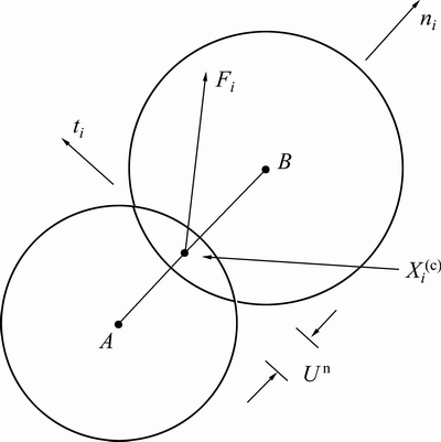
Fig. 6 Schematic diagram of linear ball-ball contact in PFC2D

If Uⁿ≤0 (a gap exists), then both normal and shear forces are set to zero, otherwise the contact is checked for slip conditions by calculating the maximum allowable shear contact force:

                               (8)

where μ is the friction coefficient between grains.

If >, then slip is allowed to occur (during the next calculation cycle) by setting the magnitude of  equal to . The basic theory and specific functions of PFC are described in more details in Ref. [26].

The PFC model needs to set micro-mechanical parameters instead of assuming the material constitutive relationship beforehand. A typical PFC^2D model requires the following micro-mechanical parameters: particle radius, normal and shear stiffness of the particle contacts, friction coefficient between particles and normal and shear strength of particle bonds. Since these micro- mechanical parameters cannot be measured directly during laboratory tests, numerical calibration was required to let rock model get ideal macro-properties, such as uniaxial compressive strength, elastic modulus, and Poisson ratio. The numerical uniaxial compressive test (Fig. 7) and biaxial-test are common methods for numerical calibration.

In PFC, the real-time contact searching logic makes it very convenient for the studies on dynamic impacts and crack evolution of rocks [26].

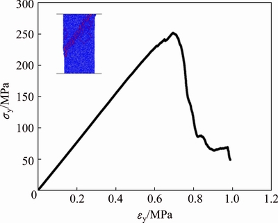
Fig. 7 Numerical result of uniaxial compression test with PFC^2D

4.2 Numerical model

Numerical SHPB models were established according to the laboratory SHPB tests. All the components of the SHPB system in laboratory were simulated by analogue objects in the software. Previous numerical studies revealed that short elastic bars could be used without affecting the test accuracy when special shape strikers were used for SHPB tests [20,22], so the length of the input and output bars in the numerical models were both selected to be 1.5 m. The stress monitoring points were set in the middle of the input and output bars, which could give stress/strain information for the further calculation as in laboratory tests. The special-shape striker was also modeled [17,22]. Since the calculation can be stopped before the tensile wave from the end of output bar arrives the specimen, the absorption bar was not modeled in the numerical environment. As the three representative specimens #1, #2 and #3 had similar geometric parameters, which can be seen from Table 1, the same specimen geometry was used in the numerical model with a diameter of 49.9 mm and a height of 50 mm. Then the analogue specimen was applied with the loading conditions as the laboratory tests. The counterpart specimens in simulation were called analogue specimens #1, #2 and #3, respectively.

The overall model of the numerical SHPB test can be seen in Fig. 8. On the contact sides of the specimen, the striker, and the elastic bars, a special alignment of the numerical particles was conducted to improve the contact condition [20]. The numerical modeling procedure includes the following three steps [20,26]. Firstly, the shape and location of model components were defined by a series of frictionless walls. Secondly, the radius expansion method was applied to generate particles to filled spaces which are defined by walls. The size distribution of the particles satisfies a uniform distribution with specified values of minimum and maximum radii. Finally, the micro-parameters of the different model components were assigned to corresponding particles and contacts.

The determination of the micro-parameters of the PFC models usually needs a numerical calibration. For the numerical SHPB test, the calibration consists of the following steps.

1) Determining the parameters of analogue striker and elastic bars. According to the mass conservation law and previous simulation experience [20], the micro- parameters of the steel bars and the striker were taken directly as Table 2. The bond strength of bar particles was selected to be extremely high, because the strength of the bars was very high and no damage would happen in bars during the tests [20]. The SHPB tests with no specimen (Fig. 8(a)) were done to check the system response. Figure 9(a) shows the comparison between the incident waves of laboratory test and numerical test when the striker’s impact velocity is 10 m/s. It can be seen that the chosen micro-parameters of the analogue striker and input bar can ensure the reproduction of the laboratory results. It should be mentioned that the initial time of the incident waves of the simulation and experiment tests in Fig. 9(a) have been shifted to overlay for comparison.

2) Determining the parameters of analogue specimen. In PFC, there is a standard calibration procedure for choosing the micro-parameters of specimens [26]. The geometrical parameters of the particles including the particle radius and porosity, which are the major determinants of the calculation accuracy and efficiency, were firstly chosen to be 0.3-0.9 mm and 0.02, respectively [20]. With these parameters, numerical tests were carried out and several groups of micro- mechanical parameters were selected by trial and error to reproduce the macro-mechanical behavior of the specimens in laboratory [26]. In detail, the micro- deformational parameters, i.e., the normal and shear contact stiffness were mainly calibrated according to the elastic modulus and Poisson ratio, while the micro- strength parameters, i.e., the normal and shear strengths were closely linked to the uniaxial compression strength of the specimen. To consider the heterogeneity of rock properties, the micro-strength parameters were assumed to obey a normal distribution. Numerical dynamic experiments were then conducted under these groups of micro-parameters. One group of them, which can realize the best fit with the stress-strain curves obtained from the SHPB tests in laboratory, was selected as the final micro-parameters of particles (Table 2). The good consistency of the numerical and experimental results as shown in Fig. 9(b) verifies the applicability of the numerical model to reveal the micro-behavior of specimens that cannot be monitored in laboratory.

4.3 Micro-fracturing at different strain rates

In PFC, there are two failure patterns of particles bonded together: tensile failure and shear failure (Figs. 10(a) and (b)). When the internal stresses exceed the critical normal or shear strength of the particle contacts, micro-cracks can be found and denoted by the code. A tensile crack initiates when normal stress acting on contact point is greater than its normal strength, whereas a shear crack initiates when a bond’s shear strength is exceeded.

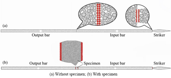
Fig. 8 Numerical SHPB model and contact condition between different parts

Table 2 Micro-parameters of PFC model

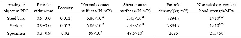
Fig. 9 Result comparison between numerical and laboratory tests

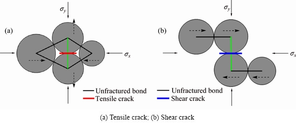
Fig. 10 Schematic diagrams of crack generation

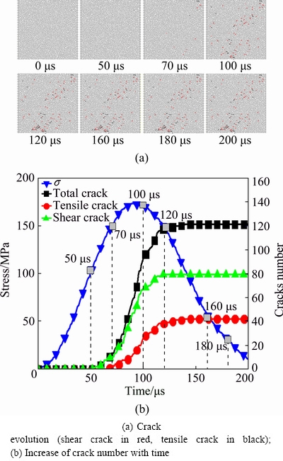
Fig. 11 Numerical results of analogue specimen #1

Figure 11(a) shows the crack evolution of the analogue specimen #1. Almost no cracks were found in the specimen during its elastic deformation before 50 μs. Then cracks accumulated gradually but distributed only at limited areas of the specimen. Figure 11(b) quantitatively gives the number of tensile cracks and shear cracks. Shear cracks emerged at 50 μs, and tensile cracks emerged around 70 μs. The tensile and shear cracks both stopped increasing at around 120 μs. It is notable that the number of tensile cracks was less than the number of shear cracks all the time at this strain rate.

Figure 12(a) shows the crack evolution of the analogue specimen #2. It can be seen that the density of the cracks began to increase near 80 μs, when the specimen deformed to its peak strength. Cracks penetrated the specimen at about 140 μs, and this result was in accordance with the laboratory phenomenon shown in Fig. 3(c). Figure 12(b) shows that the number of cracks in the specimen increased very quickly at the post-failure stage in this case, especially for tensile cracks. In this case, the final cracks quantity in analogue specimen #2 was tenfold more than the number of cracks of analogue specimen #1. There were two features of crack evolution in Fig. 12: 1) the number of the tensile cracks increased continually during the deformation, and the number of the shear cracks only increased to a certain amount; 2) shear cracks predominated at first, then the number of tensile cracks increased rapidly and exceeded the number of the shear cracks.

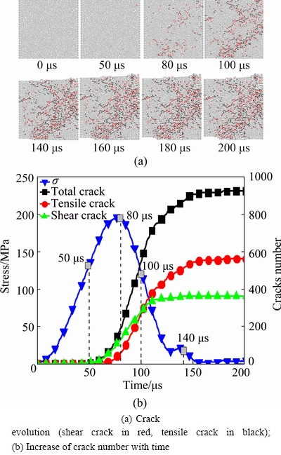
Fig. 12 Numerical results of analogue specimen #2

Figure 13(a) gives the results of the analogue specimen #3. More intensive cracks could be observed in this case compared to analogue specimens #1 and #2. Figure 13(b) also shows that shear cracks appeared first and the number of them would increase to a certain value. The tensile crack appeared lately and its number was less than that of shear crack before the peak strength. After the peak strength, tensile cracks would outnumber shear cracks and they could increase continuously till the final failure stage.

Figures 11-13 exhibit some interesting information about the crack evolution during the failure process of rocks. The shear cracks always appeared earlier than tensile cracks in all case. The number of shear cracks was greater than the number of tensile cracks all the time in the test of analogue specimen #1, but the quantity of tensile cracks exceeded shear cracks number during the post-peak stage in the tests of analogue specimens #2 and #3. It can be seen from Figs. 2-4 that few visible cracks appeared on sample surface before the peak stress in all laboratory tests. During the post-peak stage, some visible cracks closed gradually on specimen #1, while visible cracks propagated along the axial direction on specimens #2 and #3.

For rock specimen, the inner grains bond closely at nature state. Under external load, the grains would adjust their position. Then the relative slip, or shear crack, could be triggered. It is the reason why shear cracks appeared firstly in all cases. When the specimen had some shear cracks, rock grains in it did not bond as closely as before.

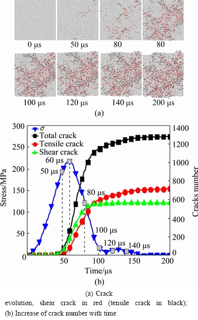
Fig. 13 Numerical results of analogue specimen #3

With the increase of external load, some of the inner grains tried to separate from each other. Once the stress between any adjacent grains exceeding their normal bond force, tensile failure happened and tensile cracks appeared.

Although the strain rate effect of rock and the appearance of micro-cracks were simulated by PFC^2D, the micro-crack distribution of simulation did not match completely with macro-cracks observed on cylindrical specimen surface of laboratory tests. The reason of this phenomenon is that a two-dimensional square is the projection of a cube rather than a cylinder in numerical simulation. The PFC^3D software is suggested to get realistic simulation effect if necessary, but the computing time has to be extended because the number of balls in the particle model increases.

5 Conclusions

1) Dynamic tests of granite specimens were conducted at different strain rates and the stress state and crack development of specimens at post failure stage had been monitored. The test results showed that the SHPB principles of stress equilibrium could be well satisfied even when visible cracks existed in specimens during the post failure stage.

2) Based on high-speed images, visible cracks always began to appear after the peak stress and could be classified as two groups. One group of cracks emerged from the side of the specimen and spread along the loading direction. The other group of cracks formed at the contact ends between the steel bar and the specimen, and then connected each other as a ring shape. With the increase of the impact loading, cracks accumulated more intensively.

3) The numerical simulation by means of PFC^2D demonstrated that the failure process of rock can be regarded as the generation and evolution of micro-cracks (including shear and tensile cracks), and the crack density of specimen increased with the strain rate. In dynamic compressive test, shear cracks always appeared firstly. Then a large number of tensile cracks followed and ultimately caused visible cracks on the surface of specimen.

References

[1] COOK N G W. The failure of rock [J]. International Journal of Rock Mechanics and Mining Science, 1965, 2(4): 389-403.

[2] SALAMON M D G. Stability, instability and design of pillar workings [J]. International Journal of Rock Mechanics and Mining Science and Geomechanics Abstracts, 1970, 7(6): 613-631.

[3] BARNARD P R. Researches into the complete stress-strain curve for concrete [J]. Magazine of Concrete Research, 1964, 16(49): 203-210.

[4] WAWERSIK W R, FAIRHURST C. A study of brittle rock fracture in laboratory compression experiments [J]. International Journal of Rock Mechanics and Mining Science and Geomechanics Abstracts, 1970, 7(5): 561-575.

[5] WAWERSIK W R, BRACE W F. Post-failure behavior of a granite and diabase [J]. Rock Mechanics, 1971, 3(2): 61-85.

[6] HUDSON J A, CROUCH S L, FAIRHURST C. Soft, stiff and servo-controlled testing machines: A review with reference to rock failure [J]. Engineering Geology, 1972, 6(72): 155-189.

[7] ZHOU Ying-xin, ZHAO Jian. Advances in rock dynamics and applications [M]. Boca Raton: CRC Press, 2011.

[8] FIELD J E, WALLEY S M, PROUD W G, GOLDREIN H T, SIVIOUR C R. Review of experimental techniques for high rate deformation and shock studies [J]. International Journal of Impact Engineering, 2004, 30(7): 725-775.

[9] ZHANG Q B, ZHAO J. A review of dynamic experimental techniques and mechanical behaviour of rock materials [J]. Rock Mechanics and Rock Engineering, 2014, 47(4): 1411-1478.

[10] GAMA B A, LOPATNIKOV S L, GILLESPIE J W. Hopkinson bar experimental technique: A critical review [J]. Applied Mechanics Reviews, 2004, 57(4): 223-250.

[11] GRANGE S, FORQUIN P, MENCACCI S, HILD F. On the dynamic fragmentation of two limestones using edge-on impact tests [J]. International Journal of Impact Engineering, 2008, 35(9): 977-991.

[12] DAI Feng, HUANG Sheng, XIA Kai-wen, TAN Zhuo-ying. Some fundamental issues in dynamic compression and tension tests of rocks using split Hopkinson pressure bar [J]. Rock Mechanics and Rock Engineering, 2010, 43(6): 657-666.

[13] LI Xi-bing, ZHOU Zi-long, HONG Liang, YIN Tu-bing, GONG Feng-qiang. Large diameter SHPB tests with a special shaped striker [J]. ISRM News Journal, 2009, 12: 76-79.

[14] ZHOU Zi-long, LI Xi-bing, YE Zhou-yuan, LIU Ke-wei. Obtaining constitutive relationship for rate-dependent rock in SHPB tests [J]. Rock Mechanics and Rock Engineering, 2010, 43(6): 697-706.

[15] CHEN W W, SONG B. Split Hopkinson (Kolsky) bar: Design, testing and applications [M]. New York: Springer, 2011.

[16] LI Xi-bing, ZHOU Zi-long, LIU De-shun, YIN Tu-bing. Wave shaping by special shaped striker in SHPB tests [C]//ZHOU Ying-xin, ZHAO Jian. Advances in rock dynamics and applications. Boca Raton: CRC Press, 2011: 105-124.

[17] ZHOU Y X, XIA K, LI X B, LI H B, MA G W, ZHAO J, ZHOU Z L, DAI F. Suggested methods for determining the dynamic strength parameters and mode-I fracture toughness of rock materials [J]. International Journal of Rock Mechanics and Mining Sciences, 2012, 49: 105-112.

[18] PIERRON F, FORQUIN P. Ultra-high-speed full-field deformation measurements on concrete spalling specimens and stiffness identification with the virtual fields method [J]. Strain, 2012, 48(5): 388-405.

[19] ZHANG Q B, ZHAO J. Determination of mechanical properties and full-field strain measurements of rock material under dynamic loads [J]. International Journal of Rock Mechanics and Mining Sciences, 2013, 60: 423-439.

[20] LI Xi-bing, ZOU Yang, ZHOU Zi-long. Numerical simulation of the rock SHPB test with a special shape striker based on the discrete element method [J]. Rock Mechanics and Rock Engineering, 2014, 47(5): 1693-1709.

[21] ZHOU Zi-long, LI Xi-bing, ZOU Yang, JIANG Yi-hui, LI Guo-nan. Dynamic Brazilian tests of granite under coupled static and dynamic loads [J]. Rock Mechanics and Rock Engineering, 2014, 47(2): 495-505.

[22] ZHOU Zi-long, LI Xi-bing, LIU Ai-hua, ZOU Yang. Stress uniformity of split Hopkinson pressure bar under half-sine wave loads [J]. International Journal of Rock Mechanics and Mining Sciences, 2011, 48(4): 697-701.

[23] BIENIAWSKI Z T, BERNEDE M J. Suggested methods for determining the uniaxial compressive strength and deformability of rock materials [J]. International Journal of Rock Mechanics and Mining Sciences and Geomechanics Abstracts, 1979, 16(2): 138-140.

[24] POTYONDY D O, CUNDALL P A. A bonded-particle model for rock [J]. International Journal of Rock Mechanics and Mining Sciences, 2004, 41(8): 1329-1364.

[25] HAZZARD J F, YOUNG R P, MAXWELL S C. Micromechanical modeling of cracking and failure in brittle rocks [J]. Journal of Geophysical Research: Solid Earth, 2000, 105(B7): 16683-16697.

[26] Itasca Consulting Group Inc. Pfc2d user’s manual, version 4.0 [M]. 4th ed. Minneapolis: Itasca Consulting Group Inc, 2008.

基于SHPB实验的岩石峰后动态行为研究

周子龙¹，赵 源¹，江益辉²，邹 洋³，蔡 鑫¹，李地元¹

1. 中南大学 资源与安全工程学院，长沙 410083；

2. 中国中铁工程设计咨询集团有限公司，北京 100000；

3.  Polytechnique  de Lausanne (EPFL), School of Architecture, Civil and Environmental Engineering, Lausanne CH-1015, Switzerland

摘  要：运用改进的SHPB实验系统开展岩石动态力学试验，借助高速摄影仪和动态应变仪组成的同步测量装置研究岩石在冲击荷载下的破坏过程和内在机制。结果表明：在峰后阶段，尽管岩样已经产生了可见的裂隙但仍能保持很好的应力平衡状态。岩样被劈裂成条状后依然能承受一定的外应力并保持两端的应力平衡。同时，进一步的颗粒流数值模拟显示，岩石的破坏过程可以用微观破裂的演化来描述。剪切裂隙总是最先出现并在外部应力下降到一定水平时停止增长。然而，拉伸裂隙在岩样所受应力接近其强度峰值时出现，并对最终的破坏形态起决定性的影响。

关键词：岩石动力学；峰后破坏；应力平衡；裂隙演化；颗粒流程序

(Edited by Yun-bin HE)

Foundation item: Project (2015CB060200) supported by the National Basic Research and Development Program of China; Projects (51322403, 51274254) supported by the National Natural Science Foundation of China

Corresponding author: Zi-long ZHOU; Tel: +86-13787202629; E-mail: zlzhou@csu.edu.cn

DOI: 10.1016/S1003-6326(17)60021-9