J. Cent. South Univ. (2012) 19: 593-599

DOI: 10.1007/s11771-012-1044-z

Rapid identification of single constant contaminant source by

considering characteristics of real sensors

CAI Hao(蔡浩)^{1, 2}, LI Xian-ting(李先庭)¹, KONG Ling-juan(孔令娟)³,

MA Xiao-jun(马晓钧)¹, SHAO Xiao-liang(邵晓亮)¹

1. Department of Building Science, School of Architecture, Tsinghua University, Beijing 100084, China;

2. Engineering Institute of Engineering Corps, PLA University of Science & Technology, Nanjing 210007, China;

3. Nanjing Artillery Academy, Nanjing 211132, China

? Central South University Press and Springer-Verlag Berlin Heidelberg 2012

Abstract: For the release of hazardous contaminant indoors, source identification is critical for developing effective response measures. A method which can quickly and accurately identify the position, emission rate, and release time of a single constant contaminant source by using real sensors was presented. The method was numerically demonstrated and validated by a case study of contaminant release in a three-dimensional office. The effects of the measurement errors and total sampling period of sensor on the performance of source identification were thoroughly studied. The results indicate that the adverse effects of the measurement errors can be mitigated by extending the total sampling period. For reaching a desirable accuracy of source identification, the total sampling period should exceed a certain threshold, which can be determined by repeatedly running the identification method until the results tend to be stable. The method presented can contribute to develop an onsite source identification system for protecting occupants from indoor releases.

Key words: source identification; contaminant source; indoor environment; computational fluid dynamics (CFD); air distribution

1 Introduction

In the cases when hazardous contaminants were released in indoor environments, such as the biochemical terrorist attacks, epidemic outbreak, and toxic gas leakage, quick and accurate identification of contaminant source is crucial to take prompt and proper responses for protecting occupants and mitigating losses. The identification of source in heat transfer, groundwater transport, and atmospheric constituent transport has been extensively studied [1-4]. In contrast, only a few studies have been conducted on the identification of indoor contaminant source. A comprehensive review of the source identification methods used in both groundwater and air fields indicated that great challenges remain to be overcome in the air field due to the significant differences between the two types of problems [5].

With increasing concerns regarding the hazards of indoor contamination, several studies have been devoted to the identification of indoor contaminant source in recent years. For identifying the contaminant source in the buildings with many compartments, several methods have been presented, such as Bayesian probability model [6], genetic algorithm [7], and probability-based inverse multi-zone model [8]. In these studies, the airflow and contaminant transport were calculated using multi-zone models [9], which can only provide macroscopic information about the contaminant transport. Thus, these studies can hardly provide exact position and emission rate of contaminant source. For identifying the contaminant source more accurately in single space, several methods based on inverse computational fluid dynamics (CFD) modeling have been presented, such as inverse CFD model with quasi-reversibility (QR) method [10] and that with pseudo-reversibility (PR) method [11], and probability-based CFD modeling method [12].

The above studies have greatly promoted the development of source identification methods for indoor environment applications. However, only a little progress has been made to identify sources by considering the characteristics of real sensors, which is critical for developing an onsite source identification system in real-world buildings. When real sensors are used, there are primarily three challenges faced with source identification, including: 1) the losses of concentration below the threshold of sensors, 2) the noises existing in measurements, and 3) the release time of source, an important information for source identification. As a preliminary attempt to overcome these challenges, this work aims to develop a method which can quickly identify the position, emission rate, and release time of a single constant contaminant source by considering the characteristics of real sensors. The method is numerically demonstrated and validated by identifying a contaminant released in a three-dimensional office. The performances of the method are tested and compared by using different levels of measurement errors and total sampling periods.

2 Source identification method

2.1 Basic assumptions

The problem concerned is specified with the following assumptions:

1) The problem is the dispersion of passive gas in steady-state indoor airflow field. For most ventilated indoor environments, the airflow field can reach steady-state much faster than the dispersion of contaminant. Usually, the airflow is turbulent and the contaminant concentration is low. Thus, the contaminant dispersion primarily depends on the flow characteristic regardless of contaminant type and has trivial effects on the airflow field.

2) The number of potential sources is limited and their locations are known. This assumption can cover a variety of indoor contaminant dispersion scenarios, such as the virus-spreading from patients at certain positions, hazardous agents released by terrorists from supply air inlets, and the leakage of toxic gas from certain locations.

3) Only a single source with constant emission rate is continuously released. This work only considers continuous releases which are more common than instantaneous releases in practice. The assumption is still applicable for the continuous releases with changing rates, if the change is slow and the identification process is quick enough.

4) A limited number of real sensors are used. With real sensors, sophisticated identification methods are needed to address the problems of data missing and measurement errors.

With the above assumptions, a source identification method is developed based on an analytical expression of transient contaminant dispersion presented in our previous studies [13-14]. By virtue of the analytical expression, the method only needs running a limited number of CFD simulations (equal to the number of potential source locations) before the release event. Each CFD simulation covers a scenario in which only one of the potential sources is released at a nominal emission rate. After the limited number of CFD simulations, the method can identify the position, emission rate, and release time of a single constant source in real-time using real sensors during the event.

2.2 Analytical expression of transient contaminant dispersion

For the dispersion of passive gas in steady-state airflow field, the transient concentration of contaminant at arbitrary indoor point p can be expressed as [13-14]

         (1)

where C_{S, k} is the concentration of the k-th inlet, C₀ is the initial concentration, S_i is the emission rate of the i-th source, Q is the air flow rate, a_{S, k-p}(t) is the transient accessibility of supply air (TASA) from the k-th inlet to point p at moment t, a_{C, i-p}(t) is the transient accessibility of contaminant source (TACS) from the i-th source to point p at moment t; K and I are the numbers of the inlets and sources, respectively.

The TASA from the k-th inlet to any indoor point p at moment t is defined as [13-14]

                            (2)

The TACS from the i-th source to any indoor point p at moment t is defined as [13-14]

                            (3)

where C_{e, i} is the average exhausted concentration under steady-state conditions.

TASA quantifies the effect of supply air on an indoor position at different moments. It is a function of the flow characteristic regardless of contaminant type and source. In contrary, TACS quantifies the effect of contaminant source on an indoor position at different moments. It is a function of both the flow characteristic and the source location regardless of emission rate and contaminant type.

With the analytic expression, only the TASA from each inlet and the TACS from each source need to be calculated by time-consuming CFD simulations. With the calculated TASA and TACS, the transient contaminant distribution under different concentrations of supply air inlets and emission rates of sources can be quickly obtained by simple algebraic calculation (see Eq. (1)). This feature of the analytic expression provides a foundation for simulating the dispersion of contaminant or identifying the characteristics of sources in real time.

2.3 Modeling of source identification

Assume that there are N potential contaminant sources and M sensors indoors. The i-th contaminant source and the j-th sensor are denoted as C_i and S_j, respectively.

The TACS from each potential contaminant source to each sensor within time period τ₁ can be obtained using CFD. With Eqs. (3) and (4), the TACS from the i-th source to the j-th sensor at moment t is

                          (4)

where S is the emission rate of source used in CFD simulations, C_j(t) is the calculated concentration at the j-th sensor and moment t.

Equation (4) can be transformed to an array with N₁ elements by discretizing τ₁ into N₁ moments with an interval ?t:

             (5)

where , and N₁= τ₁/?t.

At moment t_s=0 s, one of the potential sources S_L is released at a constant rate . The presence of contaminant is first detected by the k-th sensor R_k at moment . The sensor is called the first responding sensor (FRS) and  is called the lag time of the FRS. Then, the problem is how to identify the , , and  using the measurements of FRS.

Assume that the total sampling period of the FRS  is τ₂ (τ₂≤τ₁-). With an sampling interval ?t, N₂ measurements of the FRS can be expressed by an array as follows:

                     (6)

where  is the measurement of sensor R_k at moment .

Extract N₂ elements from the j-th element of array a_{C, i-k} to construct a new array as

                (7)

where  is the TACS from the i-th source to the K-th sensor at moment j×?t.

To identify the lag time , an index called scale of lag time (SLT) is defined as

              (8)

where STD(·) is a function to calculate the standard deviation of an array, mean(·) is a function to calculate the mean value of an array. The SLT index T_{i, j} quantifies the correlation degree between C_k and A_{i, j}. The greater the value of T_{i, j} is, the higher the correlation degree is between the two arrays.

Further define an index called scale of source position (P) as

                            (9)

For N potential contaminant sources, an array of P_i can be written as

                          (10)

If the -th element is the maximum of P, then it is indicated that a maximum correlation degree can be reached between C_k and , which further indicates that the -th element in array (S₁, S₂, …, S_N) is the source to be identified.

After the position of source is determined, the lag time of sensor R_k can be identified by searching the maximum element in the following array:

                  (11)

If the -th element is the maximum of T_L, then it is indicated that a maximum correlation degree can be reached between C_k and . Thus, the lag time of R_k is

                                (12)

When the initial concentration is 0, all the inlet concentrations are 0, and only a single source is released indoors. The analytical expression of transient contaminant dispersion (Eq. (1)) can be reduced to

                         (13)

By using Eq. (13), with the identified source position and lag time of FRS, the emission rate of source can finally be determined as

                   (14)

2.4 Procedure of source identification

The procedure is summarized as follows:

1) Calculate the steady-state flow field using CFD;

2) Calculate the distribution of TACS for each potential source using CFD;

3) Solve the indices T (Eq. (8)) and P (Eq. (9));

4) Identify the location of source and the lag time of FRS with calculated T and P;

5) Solve the emission rate of source (Eq. (14)).

In practice, the time-consuming CFD simulations in Steps 1 and 2 can be conducted before the contaminant release event, and Steps 3, 4, and 5 can be completed quickly during the event.

3 Case study

3.1 Case setup

The office room under study (Fig. 1) was 9.6 m long (X), 3.2 m high (Y), and 5 m wide (Z) and was ventilated with two supply air inlets (0.4 m×0.4 m) and an exhaust air outlet (0.8 m×0.4 m). The supply air was 0.128 m³/s and 16 °C. The heat generation rates of each computer, person, and lamp were 108, 75, and 34 W, respectively, while the window contributed 220 W. For simplicity, the envelope of room was assumed as adiabatic boundary.

Each of the six persons in the room was sitting at a fixed place. The potential virus sources corresponding to each person were numbered as S₁–S₆ (Fig. 1(b)). Assume that only S₁ was spreading virus. As the source would be identified in short time compared with the development of disease, the emission rate of S₁ was as a constant of 50 units/s. Five virus sensors (R₁–R₅) were installed in the office (Fig. 1). The threshold of each sensor is 1 unit/m³. The positions of the sensors and potential sources are summarized in Table 1.

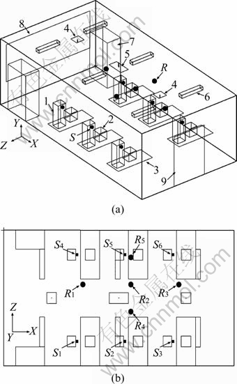
Fig. 1 Schematic diagrams of office room: (a) Three- dimensional sketch map; (b) Plane layout (1-Person; 2-Computer; 3-Table; 4-Supply air inlets; 5-Exhaust air outlets; 6-Lamp; 7-Cabinet; 8-Window; 9-Door; Contaminant sources: S₁–S₆; Sensors: R₁–R₅)

Table 1 Positions of sensors and potential virus sources

3.2 Simulation tool

A commercial CFD program AIRPAK is used as simulation tool, which is customized from a general-purpose program FLUENT for indoor environment simulations. The AIRPAK has been validated by numerous indoor airflow and contaminant dispersion studies, as reported in Ref. [15]. A zero-equation turbulence model [16] was employed to account for the indoor turbulent flow. The momentum equations were solved on non-uniform staggered grids by using a semi-implicit method for pressure-linked equations (SIMPLE) algorithm [17]. The room was discretized by 56 244 hexahedral control volumes which were systematically refined to ensure that the solution was grid independent.

3.3 Procedure of validation

Validation was performed in the following steps:

1) Calculate the steady-state flow field using CFD;

2) Calculate the distributions of TACS for six potential sources by six CFD simulations;

3) Simulate the dispersion of source S₁ at a rate of 50 units/s using CFD. Set the threshold for each sensor as 1 unit/m³ and find out the FRS and its lag time.

4) Test the identification method by using inputs: (1) simulated concentrations above 1 unit/m³ at the position of FRS (called exact measurements of the FRS); (2) exact measurements perturbed with a low level of white Gaussian noises, and (3) a high level of white Gaussian noises;

5) Evaluate the results.

4 Results and discussion

4.1 Results of CFD simulations

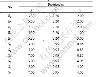
The steady-state flow field was calculated at first. Figure 2 shows the airflow pattern on a vertical plane through the centerline of the inlets. The supply air was injected from the two inlets to the floor, then flowed along the floor and created several vortexes, and finally was vented out from the outlet.

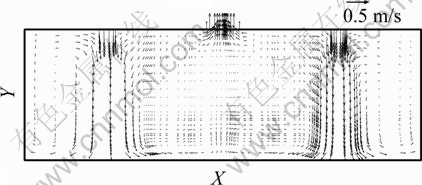
Fig. 2 Airflow pattern on vertical plane through centerline of inlets (Z=2.5 m)

Followed by the calculation of flow field, the dispersion of contaminant over 180 s from each potential source was simulated. In this case, six CFD simulations were conducted and the emission rate of the source was 100 units/s for each simulation. As an example, the concentration distributions on a horizontal plane through sensors for the release of source S₁ at different moments are plotted in Fig. 3.

Fig. 3 Concentration distributions on horizontal plane through sensors (Y=2.2 m) for release of source S₁ at different moments: (a) 30 s; (b) 120 s

After the six CFD simulations, the TACS from each potential source to each sensor can be easily calculated using Eq. (5). The variations of TACS from six potential sources (S₁–S₆) to sensor R₁ are plotted in Fig. 4.

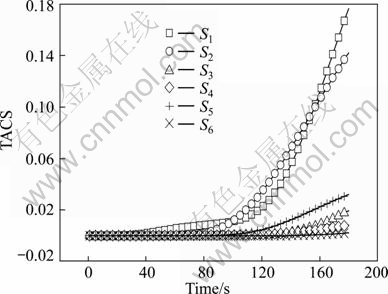
Fig. 4 Transient accessibility of contaminant source (TACS) over time from potential sources (S₁–S₆) to sensor R₁

The release of source S₁ at 50 units/s was simulated by CFD again to test the identification method presented. By setting 1 unit/s as threshold for each sensor, it is obtained that the FRS was R₁ and its lag time was 43 s.

4.2 Source identification with exact measurements

The simulated concentrations above 1 unit/m³ at the position of R₁ were called the exact measurements of the FRS. The identification method was tested with exact measurements for different total sampling periods of R₁. All the calculations were conducted on a personal computer (CPU: Intel(R) Core(TM)2 T7200 @ 2.00 GHz). The results of identification are listed in Table 2. When the total sampling period was 30 s, although the position of source was correctly determined, there were great discrepancies in the results of the emission rate of source and the lag time of R₁. When the total sampling period was larger than 35 s, the identification results were extraordinarily accurate. A possible explanation for such a high accuracy is the use of exact measurements in this case. In addition, the computing time of each case was very short (around 0.1 s). The above results indicate that, if the total sampling period of sensor is long enough, the method presented has the potential to quickly and accurately identify the position, emission rate, and release time of a single constant source with the exact measurements.

Table 2 Identification results with exact measurements using different total sampling period

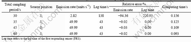
Figure 5 shows the SSP for each potential source position when the total sampling period is 60 s. The maximum value of SSP corresponds to the position of source to be identified. It is evident from Fig. 5 that the contaminant is released from S₁.

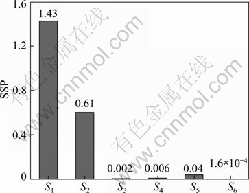
Fig. 5 Scale of source position (SSP) for each potential source position by using total sampling period of 60 s

Figure 6 shows the SLT curve for source S₁ using  60 s as total sampling period. The maximum value of the SLT curve corresponds to the lag time of FRS. There was a single peak, corresponding to 43 s, on the curve. With the SLT curve, the lag time of FRS was accurately identified (see Table 2).

4.3 Source identification with measurement errors

The identification method was further tested with measurement errors. The exact measurements of sensor R₁ were perturbed by adding two levels of normally distributed random errors (Fig. 7). The parameters of the errors are listed in Table 3.

Table 4 summarizes the identification results with the low level of noises (see Table 3). The identification results were quite incorrect and inaccurate until the total sampling period was greater than 65 s. In addition, when the total sampling period was long enough (e.g. 90 s), the results were quite accurate and very close to those listed in Table 2.

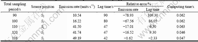
Table 5 summarizes the identification results with the high level of noises (see Table 3). A longer total sampling period (110 s) was needed to reach acceptable identification results. In addition, in comparison with the results in Tables 2 and 4, the accuracy of identifications was significantly reduced even the total sampling period used was much longer.

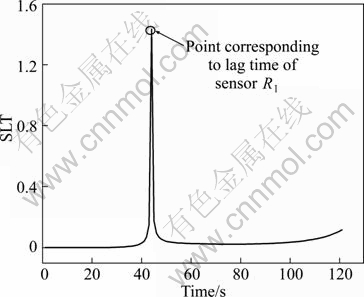
Fig. 6 Curve of scale of lag time (SLT) for source S₁ by using different total sampling periods: (a) 30 s, (b) 60s

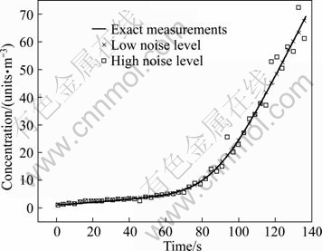
Fig. 7 Exact and perturbed measurements of first responding sensor (FRS)

Table 3 Parameters of normally distributed random errors

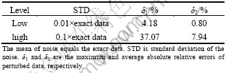
Table 4 Identification results with low noise level using different total sampling period

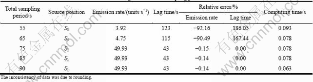
Table 5 Identification results with high noise level using different total sampling period

In summary, the above results indicate that: 1) The method has the potential to quickly and accurately identify position, emission rate, and release time of a single constant source with measurement errors; 2) The measure errors have adverse effects on the accuracy of source identification, which can be mitigated by extending the total sampling period; 3) A longer total sampling period is needed when higher level of noise is introduced in the measurements; 4) It is critical to determine a proper threshold of the total sampling period for ensuring a quick and accurate source identification.

4.4 Determination of proper total sampling period

All the results listed in Tables 2, 4, and 5 reveal that the length of total sampling period can have a great effect on the accuracy of source identification. In addition, there is a threshold of total sampling period for reaching a desirable accuracy of source identification. The method presented can be conducted on personal computer in very short time (around 0.1 s), which is much less than the total sampling period needed. In practice, the method can be conducted repeatedly with the increase of the total sampling period. A proper total sampling period can finally be determined when the identification results tend to be stable.

5 Conclusions

1) The method presented has the potential to quickly and accurately identify the position, emission rate, and release time of a single constant contaminant source indoors using real sensors.

2) The adverse effects of the measurement errors can be mitigated by extending the total sampling period of sensor. The higher the level of noise in measurements, the longer the total sampling period is needed.

3) The total sampling period should exceed a certain threshold for reaching a desirable accuracy of source identification.

4) A proper threshold of total sampling period can be determined by repeatedly running the identification method until the results tend to be stable.

References

[1] HON Y C, WEI T. A fundamental solution method for inverse heat conduction problem [J]. Eng Anal Bound Elem, 2004, 28(5): 489-495.

[2] LIU H, WU C, SHI Y. Locating method of fire source for spontaneous combustion of sulfide ores [J]. Journal of Central South University of Technology, 2011, 18 (4): 1034-1040.

[3] Atmadja J, Bagtzoglou A C. State of the art report on mathematical methods for groundwater pollution source identification [J]. Environ Forensics, 2001, 2 (3): 205-214.

[4] KOVALETS I V, ANDRONOPOULOS S, VENETSANOS A G, BARTZIS J G. Identification of strength and location of stationary point source of atmospheric pollutant in urban conditions using computational fluid dynamics model [J]. Math Comput Simulat, 2011, 82(2): 244-257.

[5] Liu X, Zhai Z. Inverse modeling methods for indoor airborne pollutant tracking: literature review and fundamentals [J]. Indoor Air, 2007, 17(6): 419-438.

[6] Sohn M D, Reynolds P, Singh N, Gadgil A J. Rapidly locating and characterizing pollutant releases in buildings [J]. J Air & Waste Manage Assoc, 2002, 52(12): 1422-1432.

[7] Arvelo J, Brandt A, Roger R P, Saksena A. An enhancement multizone model and its application to optimum placement of CBW sensors [J]. ASHRAE Trans, 2002, 108(2): 818-825.

[8] Liu X, Zhai Z J. Prompt tracking of indoor airborne contaminant source location with probability-based inverse multi-zone modeling [J]. Build Environ, 2009, 44(6): 1135-1143.

[9] Musser A. An analysis of combined CFD and multizone IAQ model assembly issues [J]. ASHRAE Trans, 2001, 107(1): 371-82.

[10] Zhang T F, Chen Q. Identification of contaminant sources in enclosed environments by inverse CFD modeling [J]. Indoor Air, 2007, 17(3): 167-177.

[11] Zhang T F, Chen Q. Identification of contaminant sources in enclosed spaces by a single sensor [J]. Indoor Air, 2007, 17(6): 439-449.

[12] Liu X, Zhai Z. Location identification for indoor Instantaneous point contaminant source by probability-based inverse computational fluid dynamics modeling [J]. Indoor Air, 2008, 18(10): 2-11.

[13] MA X, SHAO X, LI X, LIN Y. An analytical expression for transient distribution of passive contaminant under steady flow field [J]. Build Environ, 2012, 52(0): 98-106.

[14] Ma X J, Shao X L, Zhu F F, Cai H, Li X T. Experimental investigation on accessibility of supply air and contaminant source in ventilated room [C]// The 6th International Symposium on Heating, Ventilating and Air Conditioning. Nanjing, China, 2009: 873-879.

[15] Xu L. Effectiveness of hybrid air conditioning system in a residential house [D]. Tokyo: Waseda University, 2003.

[16] Chen Q, Xu W. A zero-equation turbulence model for indoor airflow simulation [J]. Energ Buildings, 1998, 28(2): 137-144.

[17] Zikanov O. Essential computational fluid dynamics [M]. Hoboken, New Jersey: John Wiley & Sons, 2011: 212-217.

(Edited by YANG Bing)

Foundation item: Project(50908128) supported by the National Natural Science Foundation of China; Project(51125030) supported by the National Science Foundation for Distinguished Young Scholars in China

Received date: 2011-07-26; Accepted date: 2011-11-14

Corresponding authors: LI Xian-ting, Professor, PhD; Tel: +86-10-62785860; E-mail: xtingli@tsinghua.edu.cn