J. Cent. South Univ. Technol. (2009) 16: 0332-0338

DOI: 10.1007/s11771-009-0056-9

Synchronous hybrid transport network design

LI Xia-miao(李夏苗)¹, ZENG Ming-hua(曾明华)¹, FU Bai-bai(傅白白)², ZHU Xiao-li(朱晓立)¹

 (1. School of Traffic and Transport Engineering, Central South University, Changsha 410075, China;

2. State Key Laboratory of Rail Traffic Control and Safety, Beijing Jiaotong University, Beijing 100044, China)

Abstract: Delay, as an inevitable real-world phenomenon, is usually ignored in transport network design. A model of urban hybrid transport system with stochastic delay was created on the basis of the idealized public transport system design. After formulating the total trip time cost composed of accessing time in the sub-region of the city, waiting time at the public transport station, and in-vehicle time in the public transit network, the analytical properties of the total trip time cost function were investigated. The results show that in the urban hybrid transport network design, the total trip time cost reaches its approximate minimum in a δ-neighbourhood of buffer time of 1.5 min, and that through modelling optimal delay in hybrid transport system, the maximal synchronization can be achieved and operational efficiency and passenger satisfaction can be improved. The proposed modelling and analytical investigations are attempts to contribute to more realistic modelling of future idealized public transport system that involves more practical constraints.

Key words: transport network design; delay; synchronization; total trip time cost

1 Introduction

Transport network design problem is of great importance and is NP-complete (NP represents non-deterministic polynomial). LOWSON [1] studied two idealized models for public transport, which were evaluated for trips via a simple linear corridor and for a more complex grid-based synchronous network system meeting a uniform travel demand and serving a whole city with a maximum of one transfer. He presented several interesting results, which are helpful for determining the basic effectiveness of a transport system as a function of network density and transport vehicle size. The models may be far from even the circumstance of the future automatic transport considering some realistic stochastic conditions.

Few literatures about the effort to handle a more detailed problem of delay in transport network design are published. It is necessary to carry out adequate studies and estimations on these problems to offer suggestion for decision-makers and practitioners before transport engineering construction.

Many researches, up to date, have been dedicated to computing optimum running timetables with a typical objective of minimizing passenger waiting time. For example, CHOWDHURY and CHIEN [2] studied how to dynamically dispatch the vehicles so as to minimize the transfer waiting time of passengers. PEDERSEN et al [3] used heuristic approaches to adjust the dispatching time of trains in a route to synchronize the timetable, which had to have constant headway. In these researches, only the planned nominal waiting time was addressed, whereas delay was neglected. At the same time, real control technique was adopted to adjust the public transport vehicle speed and waiting time period in station so as to achieve synchronization [4-5].

Resulting from the stochastic behaviour, delay cannot be avoided in practical transportation operation, especially, at peak hours. The so-called synchronization refers to the event of a connecting vehicle waiting when the feeder vehicle is late [6]. LIEBCHEN et al [7] provided the first computational study that aimed at computing delay resistant periodic timetables.

HALL et al [4] created schedule control policies to minimize transfer time under stochastic conditions, and determined how long a bus should be held at a transfer stop anticipating the arrival of passengers from connecting bus lines by assumption of the probability density function for the arrival time of a bus. FUNG et al [8] predicted the overall passenger flow for MTR’s network by means of four criteria with different weights. VANSTEENWEGEN and OUDHEUSDEN [9] tried to minimize a waiting time cost function that includes running time buffers and different types of waiting time and late arrivals.

The integration of the fixed-route transit service with some other modes such as demand-responsive service was investigated [10]. It is beneficial to taking coordination transfer into account when the variability of the arrival time of connecting buses is low. SHRIVASTAVA and O’MAHONY [5] developed feeder routes and frequencies, leading to schedule coordination of feeder buses with main transit.

The principal objective of this work is not to study on special network types or optimal routings, but to analyze the impact of multimodal transport and delay on transport system design. For that purpose, analytical models are formulated to analyze and illustrate the main mechanisms involved.

Taking delay into consideration to optimize the synchronization and to provide connectivity to customers of multiple travel patterns, the coordination between different modes is one of the challenges in operating and designing hybrid transport systems. In this work, this important problem was addressed by studying innovative methods that can reduce the total trip time cost and attain synchronization for this type of service. In particular, a grid-based hybrid transport system that integrates several modes of transport, i.e. fixed route public transit service along the grid network, and walking or bicycling in the sub-region, was studied. The transport system investigated is based on the future idealized public transport [1, 11].

2 Assumptions

The following simplifying assumptions regarding passenger flows are made.

(1) The capacity of the vehicle is sufficient at any time to receive all passengers who want to enter that vehicle. Obviously, infinite capacity is unrealistic, especially at peak hours in large cities like Paris and Tokyo. However, it is a common assumption for simplicity in transfer-scheduling practice.

(2) Passenger flow is evenly distributed. It is believed that, in practice, details of demand patterns only have second-order effects on the results.

(3) Passenger loads and bus arrival time are independent.

(4) The waiting time is the time to wait the first possible vehicle only. In other words, all the remaining passengers get on the next connecting vehicle.

(5) Passengers are inert so they prefer not transferring.

3 Models formulation

3.1 Modelling city

The studied transport system is for a city of prescribed size c (the length of side). Considering a square city may cause little loss of generality. A schematic layout of a square city and its public transport network are shown in Fig.1. The square is partitioned by the green dashed lines into n×n small zones, one of which is illustrated by the shaded square in Fig.1. All public transit links, denoted by double arrow lines, lie on a square grid, running either north-south (N-S) or east-west (E-W). There is a transport station in every zone centre that is the intersection of the transit lines.

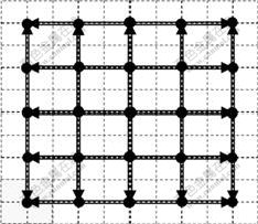
Fig.1 Schematic layout city and its public transport network

Since most important large cities now are polycentric with a dispersed travel demand pattern, and urban decay has led in some cases to “doughnut” cities such as Paris, Beijing, in which the demand for travels concentrates on rings with some distance from the old city centre, the origin and destination of trips are all assumed to be uniformly distributed within the square (service area). It is suggested that the assumption of a uniform demand over the whole city is an acceptable first approximation to many existing transport patterns. Most importantly, for the present purposes, a uniform demand might affect realization of numerical results, but it does not influence the main mechanisms that characterize the dependency between the networks of multimodal transport and the factor of delay.

3.2 Transport network formation

The transport system used to analyze this situation consists of a fixed route public transit network, and the lower-level sub-region roads providing services for the private transport mode of walking or bicycling.

The public transit network has parallel lines in both N-S and E-W directions. A series of vehicles running bi-directionally on bi-directional tracks of the fixed route public transit network accommodate to nearly identical volume of passengers who travel relatively long journey in the city.

The lower level network is just constructed by roads in each zone, namely, neo-traditional community [12]. For new urbanism, building entire residential communities is, however, very capital-intensive. It stresses a mix of compactly arranged land use in a single development with high street connectivity. Each neighbourhood has a “small town” commercial node within walking distance of most residences. The lower level roads in each zone mainly offer transport services for individuals using private modes of walking or bicycling to get to the nearest neighbouring station that locates in the community or central business district. Walking and bicycling modes might eliminate the differences in vehicle availability between the home-based and the activity-based leg of the journey, create a space of densely built form and hierarchical structure, enhance the accessibility of transport system, and thus improve attractiveness of activity-oriented transfer stations in the multimodal transport system.

Let n∈N denote the number of tracks in each direction in the public transit network and 5≤n≤40, considering the city size of our study case in Section 4 and some numerical experiments with n varying from zero to a relatively large integer. This network is an n×n grid network with station spacing S_s and line spacing S_l, satisfying S_s=S_l=c/n.

3.3 Average trip time cost in transport system

To obtain the average trip time cost in the transport system, three criteria are focused on: trip time by private mode of bicycling or walking in each lower level zone, riding time in the higher level urban public transit network, and waiting time at the station.

3.3.1 Trip time using private modes to arrive at station

The access time in the sub-region varies depending on the direction of the trip in relation to the orientation of the grid. The egress time is ignored, with no impact on the research in this paper. HOLROYD [13] gave an extensive analysis of this. Now assume that the average access distance is the function of the line spacing of the higher level network, i.e. L_a=S_l/2. The total time of access t_a can be calculated by average distance L_a, travelled by a passenger on access modes between any point in the region around the higher level network station and this station, divided by the average access and egress speed v_a.

t_a=L_a/v_a=S_l/(2v_a)=c/(2nv_a)                       (1)

Thus the trip time cost (C_a) to access the higher level can be expressed as

C_a=w_ac/(2nv_a)                                (2)

where w_a represents weight for access time.

3.3.2 Waiting time at station

The ideal running time is the smallest running time for the feeder vehicle, from its previous station to the connection station while a real running time of a vehicle will vary, depending on the circumstances. A buffer time t_b, only calculated for a connection station, is determined in order to secure a certain connection.

For the sake of simplicity, only waiting time (at stations), resulting from delay of vehicles, is involved. And to model the waiting time in the system, delay propagation is ignored between lines connecting each other at the stop.

In the scenario selected to study the transport system, it is supposed that the timetable is symmetrical. In the higher level public transit network, scheduling a transfer in one direction, for instance, eastwards, automatically schedules the transfer in the opposite direction westwards. Furthermore, a buffer time scheduled on a vehicle in eastbound direction before a transfer will appear on the vehicle in westbound direction after the transfer. In southward direction, the buffer time can be used as a maximum holding time to delay a departure, if the vehicle from next station arrives later than scheduled. Thus, introducing a buffer time for one of the vehicles involved in a transfer will suffice. In westward direction, dispatching should know for which vehicles a certain holding time is provided; furthermore, they should know the expected arrival time of the next vehicle to decide whether or not they should keep the connecting vehicle on hold.

Mainly four passenger types are influenced when a buffer time is introduced in the running time of one of the vehicles on the higher level network: transfer passengers (tr), through passengers (th), departing passengers (dep), and arriving passengers (arr). Denote the proportions of each class of passengers to the total number of passengers by P_tr, P_th, P_dep, P_arr, respectively.

In the following, an analytical expression is derived for the distribution of the resulting delay in the context of a bi-directional track in a direction to calculate the total waiting time cost in the public transit network.

Usually, passengers take the most direct route toward their destination, which is in the north, south, or east of the station. In a particular transport station, passengers shifting from a public transit line at the station and from road section in the zone where the station locates will transfer or depart from the station. Let delay D be exponentially distributed with parameter λ>0, i.e. D～E(λ).

It is assumed, for a further simplification, that along a track all delay are caused by stops of independent and identically distributed (IID) random length, and that the distances between these stops form an IID sequence.

Above all, waiting time cost for transfer passengers at a certain station is calculated. When the fixed route transit vehicles reach the station earlier than scheduled, i.e. the delay D is smaller than the buffer time t_b, the time a passenger should wait on the platform is x=t_b-D with the assumption of passengers leaving the vehicle as soon as the vehicle stops. The numerical range of t_b is assumed to be  without loss of generality, since the experiments in Section 4 reach the same results for larger value of t_b.

It was obtained that the extra time cost C_ec due to an early arrival, the waiting cost C_mc caused by missing connection, the extra time cost C_ecd of departing passengers, and the corresponding time cost C_al of arriving passengers, are as follows:

            (3)

         (4)

                        (5)

                         (6)

where w_nw denotes the weight of normally referred waiting time on a platform, w_ed is the weight for extra driving time when the scheduled running time is longer than the ideal running time, w_mc is the weight for waiting time caused by missing a connection, w_svw is the weight of waiting time while passengers are seated on a vehicle, and w_al is the weight for generalized waiting time cost in the case of arriving late at the end of a journey; and p denotes the time that transfer passengers have to wait for the next connecting vehicle, if the vehicle delay is larger than the buffer time and passengers miss the connection.

Note that an early arrival causes the extra time cost not only for transfer passengers but also for through passengers. Finally, we should be conscious of the fact that the synchronization control time of the connecting service also affects the waiting time of transfer passengers, through passengers, as well as departing passengers. The time cost of each type of passengers is the same as w_edt_b.

Assume there are all kinds of passengers in the middle station of a single-direction fixed route transit line whereas no through passengers at both ends of the line, no arriving passengers at the start end, and no departing passengers at the ending end. The total waiting time cost of a single line is thus obtained:

  (7)

Considering the 4n lines in the network, the total waiting time cost of higher level public transit network can be formulated from Eqn.(7). Thus, it is convenient to calculate the total waiting time cost C_{Total waiting} in each station of the fixed route public transit network through dividing the total cost of waiting time in the network by the total number of stations in the network:

C_{Total waiting} =

       (8)

3.3.3 In-vehicle time

It is assumed that there is an equal demand from every station to all other stations.

The average distance travelled by a passenger on a fixed route public transit vehicle can be calculated involving some simple algebra. It is convenient to evaluate the average trip length for a simple straight-line travel on the higher level public transit network. The average length of travel distance is given as follows.

For a particular fixed route public transit line, for instance, a northbound line, the total length of trip from

the ith, i=1, 2, ???, n-1, station northwards is .

The total trip length from all stops is.

The total length of all trips in the direction of N-S is B=2n²A. The total length of trips N-S and E-W is 2B.

Because the total number of travels is n²(n²-1), the average length over all trips equals 2Bn/[n²(n²-1)], which produces 2c/3 in view of S_s=c/n. Thus, the weighted riding time in the vehicle of the fixed route public transit service can be represented as

C_in-vehicle=2w_inc/(3v_i)                           (9)

where  v_i is the average in-vehicle speed of the fixed route public transit service.

3.3.4 Total trip time cost

Taking the sum of accessing time cost using private modes to get to the station area, waiting time cost in the station and the in-vehicle time cost of formulae (2), (8), and (9) respectively, presented in the above investigation, the total trip time cost (C) is

                                     (10)

4.1 Solution for formulated transport system

In this section, the relationship of minimizing the total trip time cost in the hybrid transport system with the satisfactory solutions of running time buffer and the number of public transit tracks was studied.

Some analytical properties of the total trip time cost function are presented based on the assumption that the function C(n, t_b) is continuously differentiable in relation to  and t_b in the domain ?=?{(n, t_b)│ 5≤n≤40, 0≤ t_b≤5}∈N×R⁺.

It is convenient to gain gradient for C(n, t_b), i.e., and the first order partial derivatives that are put as follows.

                 (11)

               (12)

Let c=10 km, w_nw=2.5, w_mc=2.7, w_svw=2.0, w_al=3.0, w_a=1.0, w_in=w_ed=1.0, v_a=80 m/min, v_i=1.67 v_a, p=10 min, P_tr=0.2, P_th=0.2, P_arr=P_dep=0.3, and λ=0.7.

The figure of total trip time cost function is thus exhibited in Fig.2.

Remark 1 In the case of waiting for public service, the weight is almost always expressed according to the driving time. A commonly used factor to express the value of waiting time is 2.5 [14], which means that passengers rate 1 min of waiting as equivalent to 2.5 min of driving. It has also been verified that a small change in the weight values does not make a significant difference to the buffer time estimation [9].

Remark 2 Taking the real-world passenger travel behaviour into consideration, we set the proportions of each class of passengers to the total number of passengers, i.e. P_tr, P_th, P_dep, P_arr as above. Furthermore, some experimental results when the proportions around these values are varied show that the following principal results also hold.

The relationship between ?C/?n and ?C/?t_b and   (n, t_b) is shown in Fig.3, which demonstrates that ?C/?n and ?C/?t_b are non-decreasing functions with regard to n and t_b respectively in the respective domain. The monotonicity implies that the second order partial derivatives of C(n, t_b) with regard to n and t_b respectively, i.e. ?²C/?²n and , are both non-negative.

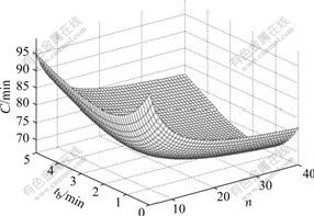
Fig.2 Total trip time cost function of hybrid transport network

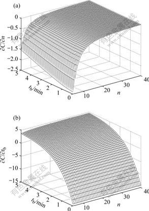
Fig.3 Relationship between of ?C/?n (a), ?C/?t_b (b) and (n, t_b)

Furthermore, computed from the given parameters, the second order mixed partial derivatives ?²C/?n?t_b and ?²C/?t_b?n, are found to be equal, as shown in following equation:

               (13)

It is observed from Fig.4 that the two mixed partial derivatives are non-negative. Hence, the Hessian matrix of total trip time cost function is positive semi-definite and total trip time cost function is convex with regard to (n, t_b). So the total trip time cost function meets the minimum at  that satisfies .

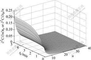
Fig.4 Relationship between the second order mixed partial derivatives and (n, t_b)

Let ?C/?t_b equal zero. It is convenient to solve the equation with the result of t_b represented by expression of n as

(100nL_w-100L_w-1 607n+347) (n-1)      (14)

where  L_w = Lambertw, and Lambertw (x) is the solution to w?exp(w)=x.

Thus, substituting the formula (14) of t_b into ?C/?n=0 yields an equation in which only one variable n is involved. Solving the equation without considering constraint condition of n generates satisfactory approximations of the number of tracks n=24.368 1 and the buffer time t_b=1.0 min with the tolerance value less than 1.0×10^-6, and the corresponding total trip time cost C=70.543 7 min. Set n=24, t_b=1.0 min, then C=71.092 8 min; and set n=25, t_b=1.0 min, then C=70.892 6 min. These two cases are acceptable for achieving satisfying urban transport service quality since the system gains its relatively small trip time cost. n=24 and n=25 correspond to neo-traditional neighbourhood with side length equal to 0.4 km or so. This result dovetails nicely with the advocated neo-traditional community. 

However, this work is not only about the acquisition of the minimal total trip time cost, but about the relationship between the total trip time cost function and number of tracks (n) and buffer time (t_b).

4.2 Optimal range of buffer time for hybrid transport network

In Section 4.1, the associations of the total trip time cost function’s first order partial derivatives ?C/?n, ?C/?t_b, and second order mixed partial derivatives with (n, t_b) are explored and the transport network that minimizes the total trip time cost is designed. Now, the relationship between the total trip time cost C(n, t_b) and (n, t_b) is investigated (see Fig.5).

Fixing the track number n, the plot of total trip time cost vs t_b is presented in Fig.5(a), which is impressively described as follows.

(1) The optimal value of t_b for attaining satisfactorily small total trip time cost and maximal synchronization is in a neighbourhood of 1.5 min N_δ={t_b:≤δ (for example, δ=0.5 min so long as n does not deviate too much from 20. There is a tendency to increase the total trip time cost if the buffer time is adjusted to smaller or larger value outside the neighbourhood.

(2) The decreasing rate of total trip time cost decreases rapidly when n approaches to about 20.

When the buffer time is fixed, it is also convenient to generate curves of the total trip time cost vs n for different values of t_b (Fig.5(b)). Fig.5(b) shows that the total trip time cost curve no longer pans down much when reaching some values of buffer time t_b. This phenomenon coincides with the above-mentioned investigation and demonstrates that there exists certain appropriate buffer time for constructing synchronous urban public transport system. For some detailed information, the bunch of plot in Fig.5(b) is enlarged in certain interval of n, for instance, [20, 25]. This further validates that the appropriate value of t_b for attaining satisfactorily small total trip time cost and maximal synchronization lies in the neighbourhood of 1.5 min.

Fig.5 Plots of total trip time cost vs t_b (a) and n (b)

5 Conclusions

(1) As a consequence of the stochastic behaviours of vehicle, delay cannot be avoided in practical operation of transportation. The impacts of multimode and delay on transport system design are principally analyzed. The analytical models of synchronous hybrid transport system with stochastic delay are developed to explore and illuminate the main mechanisms involved, and to maximize synchronization of the system.

(2) The analytical model and properties of the total trip time cost function are investigated. The total trip time cost reaches its acceptable small value and the hybrid transport system achieves its maximal synchronization with buffer time value in a δ-neighbourhood of 1.5 min, and about 24 tracks, which means that the walking or bicycling time is about 5 min for city inhabitants dwelling in the community (zone).

(3) The buffer time plays an important role in practical transport network design, infrastructure construction and traffic management. The proposed modelling approach may be a specific contribution to realistic modelling of future idealized public transport system that will become a notable aspect of transport network design in engineering practice.

References

[1] LOWSON M. Idealised models for public transport systems [J]. International Journal of Transport Management, 2004, 2(3/4): 135-147.

[2] CHOWDHURY M S, CHIEN S I. Dynamic vehicle dispatching at intermodal transfer station [C]// Proceedings of the 80th Transportation Research Board Annual Meeting, Washington DC: TRB, 2001: 3101-3108.

[3] PEDERSEN M B, NIELSEN O A, JANSSEN L N. Minimizing passenger transfer times in public transport timetables [C]// Proceedings of the 7th conference of Hong Kong Society for Transportation Studies. Hong Kong, 2002.

[4] HALL R, DESSOUKY M, LU Q. Optimal holding times at transfer stations [J]. Computers and Industrial Engineering, 2001, 40(4): 379-397.

[5] SHRIVASTAVA P, O’MAHONY M. A model for development of optimized feeder routes and coordinated schedules—A genetic algorithms approach [J]. Transport Policy, 2006, 13(5): 413-425.

[6] GOVERDE R M P. Transfer stations and synchronization [R]. Technical Report, TRAIL, Delft: Delft University of Technology, The Netherlands, 1999.

[7] LIEBCHEN C, SCHACHTEBECK M, SCH?BEL A, STILLER S, and PRIGGE A. Computing delay resistant railway timetables [R]. Technical Report TR-0066, ARRIVAL Report, Berlin: Technische Universit?t Berlin, 2007.

[8] FUNG S W C, TONG C O, WONG S C. Predicting the performance of a mass transit system by using a conventional network model [C]// Proceedings of the Croucher Advanced Study Institute (ASI) on Advanced Modeling for Transit supply and Passenger Demand. Hong Kong, Hong Kong Polytechnic University, 2004.

[9] VANSTEENWEGEN P, OUDHEUSDEN D V. Decreasing the passenger waiting time for an intercity rail network [J]. Transportation Research (Part B), 2007, 41(4): 478-492.

[10] LIAW C, WHITE C C, BANDER J J. A decision support system for the bimodal dial-a-ride problem [J]. IEEE Transactions on Systems, Man, and Cybernetics—Part A: Systems and Humans, 1996, 26(5): 552-565.

[11] PARENT M, GALLAIS G. Cybercars: Review of first projects [C]// Proceedings of the 9th ASCE International Conference on Automated People Movers (APM 03). Singapore, 2003.

[12] GUO J Y, BHAT C R. Operationalizing the concept of neighborhood: Application to residential location choice analysis [J]. Journal of Transport Geography, 2007, 15(1): 31-45.

[13] HOLROYD E M. The optimum bus service: A theoretical model for a large uniform urban area [C]// Proceedings of the 3rd International Symposium on the Theory of Traffic Flow. New York: Elsevier, 1967.

[14] WARDMAN M. Public transport values of time [J]. Transport Policy, 2004, 11(4): 363-377.

Foundation item: Project (70671008) supported by the National Natural Science Foundation of China, Project (3340-74236000003) supported by the Scientific Research Innovation Fund Project for Graduate Student of Hunan Province, China

Received date: 2008-09-29; Accepted date: 2008-11-20

Corresponding author: ZENG Ming-hua, Doctoral candidate; Tel/ Fax: +86-731-2656662; E-mail: zmhcsu@163.com

(Edited by CHEN Wei-ping)