Springback analysis and strategy for multi-stage thin-walled parts with complex geometries
来源期刊:中南大学学报(英文版)2017年第7期
论文作者:郎利辉 王耀 S. Lauridsen 阚鹏
文章页码:1582 - 1593
Key words:springback model; complex geometry; multi-stage; rigid-flexible compound process
Abstract: Springback of a SUS321 complex geometry part formed by the multi-stage rigid-flexible compound process was studied through numerical simulations and laboratory experiments in this work. The sensitivity analysis was provided to have an insight in the effect of the evaluated process parameters. Furthermore, in order to minimize the springback problem, an accurate springback simulation model of the part was established and validated. The effects of the element size and timesteps on springback model were further investigated. Results indicate that the custom mesh size is beneficial for the springback simulation, and the four timesteps are found suited for the springback analysis for the complex geometry part. Finally, a strategy for reducing the springback by changing the geometry of the blank is proposed. The optimal blank geometry is obtained and used for manufacturing the part.
Cite this article as: WANG Yao, LANG Li-hui, S. Lauridsen, KAN Peng. Springback analysis and strategy for multi-stage thin-walled parts with complex geometries [J]. Journal of Central South University, 2017, 24(7): 1582-1593. DOI: 10.1007/s11771-017-3563-0.
J. Cent. South Univ. (2017) 24: 1582-1593
DOI: 10.1007/s11771-017-3563-0

WANG Yao(王耀)1, LANG Li-hui(郎利辉)1, 2, S. Lauridsen3, KAN Peng(阚鹏)1
1. School of Mechanical Engineering and Automation, Beihang University, Beijing 100191, China;
2. Collaborative Innovation Center of Advanced Aero-Engine, Beihang University, Beijing 100191, China;
 Central South University Press and Springer-Verlag Berlin Heidelberg 2017
Abstract: Springback of a SUS321 complex geometry part formed by the multi-stage rigid-flexible compound process was studied through numerical simulations and laboratory experiments in this work. The sensitivity analysis was provided to have an insight in the effect of the evaluated process parameters. Furthermore, in order to minimize the springback problem, an accurate springback simulation model of the part was established and validated. The effects of the element size and timesteps on springback model were further investigated. Results indicate that the custom mesh size is beneficial for the springback simulation, and the four timesteps are found suited for the springback analysis for the complex geometry part. Finally, a strategy for reducing the springback by changing the geometry of the blank is proposed. The optimal blank geometry is obtained and used for manufacturing the part.
Key words: springback model; complex geometry; multi-stage; rigid-flexible compound process
1 Introduction
Springback has been a well known problem in manufacturing for many years. For simple components, techniques like overbending or stretch bending can be applied to compensate for the springback. But for the parts with complex geometries, the springback behaviour is not easily predicted and compensated for [1-3]. Meanwhile, springback is a quality concern in the metal forming industry as the shape of the final part is affected by springback ultimately. Subsequent assembly can be greatly affected if the part does not meet dimensional tolerances due to springback [4, 5]. Springback can not be avoided in die face engineering, but measures can be taken to minimize it. The most common method is springback compensation, which is done manually, i.e. measuring the springback deviation and altering the geometry of the production tools [6-8]. This is a very time-consuming and expensive process. In many cases, several correction iterations of the tools are needed. Generally, an iteration of springback correction takes five weeks and costs 70000 EUR [9, 10]. Several iterations are often needed, which significantly increases the cost and time of tool development.
Complex geometries and new materials with new properties make it very difficult to solely rely on this experience based on trial and error approach. Therefore, being able to predict springback and make design corrections before tool development and manufacturing starts can lead to savings in both cost and time. Recent development in the field of finite element analysis (FEA) has made it possible to better predict springback of complex parts. Utilizing FEA, springback can be predicted and compensated for in an easy and efficient manner [11, 12].
Austenitic stainless steel alloy, which adds mass titanium at least five times mass more than that of carbon and improves the elevated temperature properties of the alloy, is typically used in applications including exhaust systems, firewalls, boilers, welded pressure vessels, oil refinery equipment, jet aircraft components and so on. It has good formability and resistance to corrosion [13, 14]; however, a negative property of the alloy is that it suffers from more springback than does carbon steel or ferritic stainless steel does [15].
According to the springback research for parts with complex geometries, ASGARI et al [16] designed some experiments to study the sensitivity of the implicit and explicit numerical results with respect to certain arrays of user input parameters in the springback analysis of an AHSS component with complex geometries and much lower accuracies were observed in its springback predictions. The number of integration points through the thickness and tool offset was found to be of significant importance. ANDERSSON [17] developed a new semi-industrial experimental tool, flex-rail. It was a very flexible tool, which could be used for various kinds of materials, from mild steel, aluminum to advanced high strength steel by using different insert. The tool was designed for experimental analysis of 3D-springback in the more complicated automotive parts. SLOTA et al [18] described a robust method of predicting springback under bending and unbending of sheets. Constitutive models, aimed at predicting the final shape of the sheet after the springback by varying the setting of the operational parameters of the forming process, were discussed. The accuracy of the model was verified by comparison with results of PAM-STAMP 2G package and experimental results. PAPADIA et al [19] analyzed the springback phenomenon experimentally in sheet metal hydroforming. A modified approach was adopted to measure the springback of the large size part. Through the implemented methodology, it was possible to calculate the values of springback parameters. The obtained results corresponded to the observed experimental deformations. HARRISON et al [20] presented a methodology for the manufacture of tools incorporating complex surface geometry using PC-based two-and-a-half axis CADCAM systems, which might be used for component springback compensation.
The springback phenomenon has been extensively analyzed in deep drawing processes, but there are few works in the literature about springback in sheet metal multi-stage rigid-flexible compound process. Based on above research, in this work, the springback of a SUS321 complex geometry part formed by the multi-stage rigid-flexible compound process was studied through numerical simulations and laboratory experiments. In order to minimize the springback problem, an accurate springback simulation model of the part was established and validated. Following this, a strategy for producing the part within acceptable tolerances was developed.
2 Forming process analysis
2.1 Part character and used material
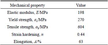
In this work, the typical part with shape and key dimensions shown in Fig. 1 is investigated. The part has a complex geometry with several sharp bends and curvatures in different directions. Springback occurs everywhere in the part, but it is most problematic in the area where the three mounting holes are located, as seen in Fig. 1(a) (marked with blue arrows). The degree of springback in angle θ3 is severe. The SUS321 austenitic stainless steel alloy sheet with an initial thickness of 0.8 mm is used, and its mechanical properties are listed in Table 1. As seen in the table, SUS321 has good formability, although higher pressures are required. And the degree of springback is more severe compared to other steel materials as its higher yield stress σs and elastic modulus E increase the springback.
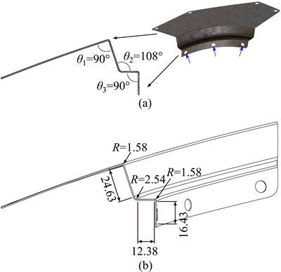
Fig. 1 Typical part with shape (a) and key dimensions (Unit: mm) (b)
Table 1 Mechanical properties of SUS321 austenitic stainless steel alloy
2.2 Numerical simulation and experimental conditions
The finite-element analysis software ETA/ DYNAFORM is applied to study the springback in combination with tests. Modern FE codes, like LS-DYNA, have shown good results for simulating formability of sheet metal. Accurate springback simulation proves to be difficult. Springback simulation is the last part of the simulation, performed after forming. Therefore, any previous errors from the forming simulation will be introduced in the springback calculations. This means that the accuracy of the springback simulation not only depends on the springback simulations itself, but also depends on the accuracy of the forming simulation.
All the experiments are conducted on the 4500 t double-action sheet hydroforming equipment, as shown in Fig. 2, in which the cavity pressure and blank holder force (BHF) can be regulated in real time according to various designed loading paths, and the maximum cavity pressure can be increased to 100 MPa and the maximum BHF can reach to 4000 kN. The dimensions of worktable are 2300 mm×1800 mm. All test conditions could be set up through the software installed in the computer integrated to the press forming machine.
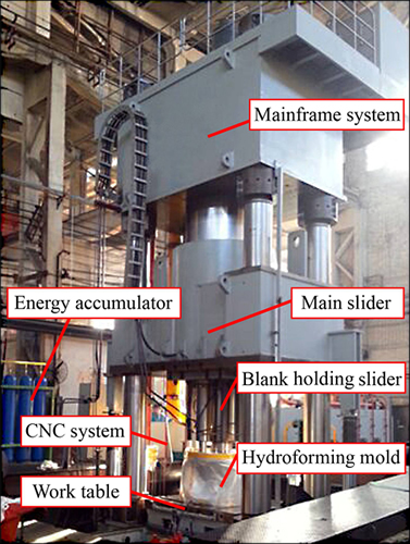
Fig. 2 4500 t double-action sheet hydroforming equipment for experiments
2.3 Sensitivity analysis of forming process
The forming process of the part applying the rigid-flexible compound process is shown in Fig. 3. In order to avoid fracture and meet the requirement of wall thickness reduction rate (only 10%), a preliminary blank shape and size designed by theoretical calculation and finite element modeling (FEM) is shown in Fig. 4. All tools are modeled as rigid bodies. Two different shell elements are used, for different purposes. Generally, the standard element type #2 Beltyschko-Tsay shell elements are used. When accurate springback results are needed, the more expensive #16 elements are used. The blanks have five or seven through-the-thickness integration points, according to the aim of simulations. Five integration points are used for the sensitivity analysis, to get a better description of the stress state through the thickness. Seven integration points are used when the result of the simulation has to be used for springback analysis. Curves for defining loads and motions are all made in Dynaform software. Symmetry has been applied to the blank, as seen in Fig. 5, to minimize computational time. A quarter of the original blank is used in the simulations.
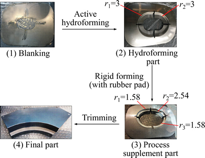
Fig. 3 Forming process of part with complex geometry (unit: mm)
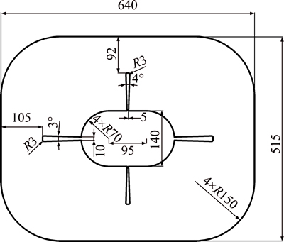
Fig. 4 Preliminary blank shape and size (unit: mm)
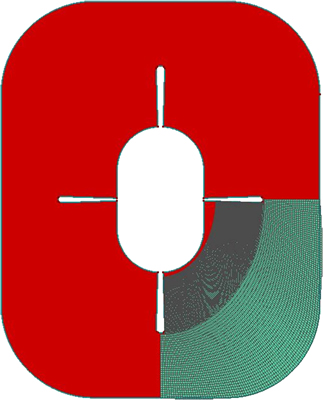
Fig. 5 Symmetry conditions applied to quarter blank during simulations
In order to meet the requirement of surface quality of the part, the active hydroforming and rigid forming with rubber pad are adopted respectively. The whole forming process includes two stages, the first one is active hydroforming. This process forms the angles θ1 and θ2. The final radii of the bends are 1.58 mm and 2.25 mm, respectively. These radii are too small to perform in one hydroforming process without risking fracturing the blank. Therefore, the radii of the bends after this hydroforming process are 3 mm. In the next rigid forming process, the radii will be formed to their final dimensions. The finite element model for the active hydroforming is shown in Fig. 6. A dummy blank with material of carbon steel Q235 is needed for the process. The dummy blank is needed because the blank has holes. Hydroforming would not be possible without the dummy blank, as there would be the same pressure above and below the blank.
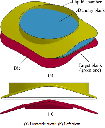
Fig. 6 FEM model of active hydroforming
The second stage is rigid forming with rubber pad, and the finite element model is shown in Fig. 7. The part undergoes two stamping processes, but at two different stations. The first stamping process gives angles θ1 and θ2 their final radii of 1.58 mm and 2.25 mm, respectively. The third bend (angle θ3) is made by the final stamping process. After treatment at this station, the blank is cut into four parts and some trimming is performed. Springback occurs after this process and it is the springback from this process that will be investigated further.
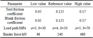
A sensitivity analysis is performed to gain a better understanding of the effects and importance of certain process parameters on the result of the simulation. An initial simulation is performed with values that will be used as reference. Next, one of the parameters will be changed to a higher value, and then a simulation is performed. Meanwhile, the same process will be done with a lower value of the same parameter. The results are compared with the reference simulation value. Table 2 lists the parameters that will be evaluated during this analysis, along with their respective values.
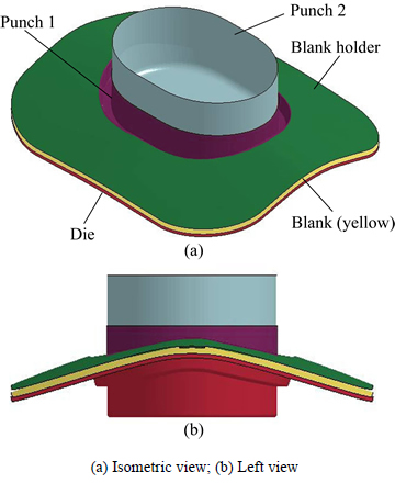
Fig. 7 FEM mode of rigid forming with rubber pad
Table 2 Parameter in sensitivity analyses and their values (values of a and b are illustrated in Fig. 9)
Stress, through the thickness of the sheet, will be evaluated in this sensitivity analysis, because stress is used directly for the springback analysis. This is done by assessing stress at the integration points through the thickness of the element. The chosen element (S 593353) for the analysis is located in an area where large springback has been reported, as seen in Fig. 8. The stress is evaluated in the element’s local x-direction. The direction is illustrated with an arrow in Fig. 8, and is in the plane of the element. The element’s local x-direction experiences larger stresses than the y-direction does, because the stresses in x-direction capture both stresses from the curvature and stretching of the blank. The y-direction is also in the plane of the element, but transverse to the x-direction. Figure 10 shows the reference stress state. Five integration points will be used for all simulations.
The stresses through the thickness of the sheet at the integration points, for different values of tool friction coefficient, blank friction coefficient, load path and binder force are shown in the Fig. 11, respectively.
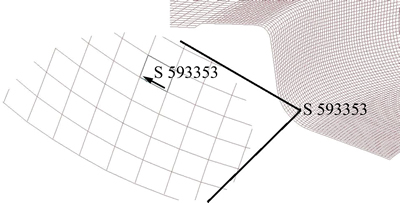
Fig. 8 Location of subject for sensitivity analysis (element 593353)
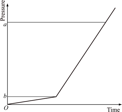
Fig. 9 Cavity pressure path from Dynaform

Fig. 10 Reference stress values at integration points for this sensitivity analysis
As seen in the figure, for the tool friction coefficient, there is a difference of 390 MPa between the highest and lowest friction values at the second integration point, while at the third integration point, the difference is 550 MPa. For the friction between the blank and the dummy blank, the maximum difference is seen at the third integration point in Fig. 11(b), where there is a difference of 275 MPa between the simulations with the high and the low values of blank friction. The cavity pressure load path shows a somewhat constant difference in stresses at the integration points in Fig. 11(c), with the maximum difference of friction values being 250 MPa at the third integration point. The load path can be changed arbitrarily, so if a certain stress start is found to be beneficial for minimizing springback, the load path is a good place to begin. No noteworthy difference in the stresses is observed from cases with the different binder forces as seen in Fig. 11(d).
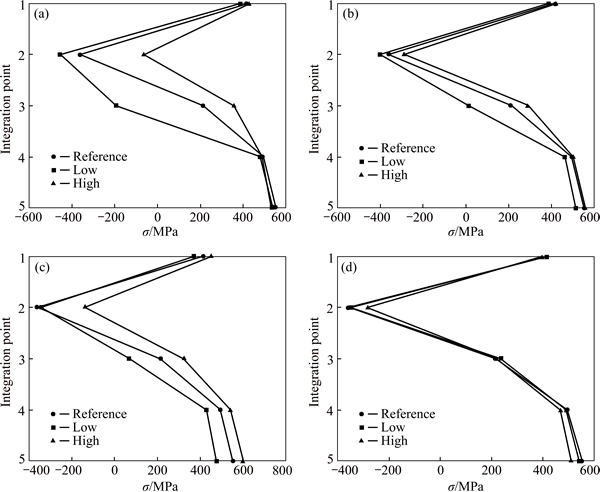
Fig. 11 Stress through thickness of sheet at integration points for different values of tool friction (a), blank friction coefficients (b), load paths (c), and binder forces (d)
Performing this analysis has provided an insight in the effect of the evaluated process parameters. The tool friction coefficient, blank friction coefficient and the cavity pressure load path are found to be of significant importance. Furthermore, evaluating stress at the integration points has given a better understanding of the stress state than that a surface contour can provide. This will be beneficial for the next springback analysis, because the input file for a springback simulation is the dynain file from the previous forming simulations. It is desirable to include as many of the forming processes as possible, to get the most comprehensive stress state in the blank.
3 Springback model
3.1 Influence of element size on springback model
Before establishing the springback model that will be used for further analysis, it is desirable to investigate how certain model factors influence the result of a springback simulation. In order to investigate the influence of the element size on springback, the forming simulations and the springback simulations will be performed with different mesh sizes, and then the results are compared. Also, it is desirable to get the lowest computational time. Three different mesh strategies are utilized, including constant mesh size, adaptive mesh size and custom mesh size.
The constant mesh size is the first strategy deployed. A constant mesh size is applied to the blank with the automatic mesh function in Dynaform, which is to be a fast indicator of analyzing how the mesh size affects the forming simulations and thereby the springback simulations. Obtaining accurate forming simulations requires a fine mesh over tool radii. Generally, at least four elements are needed around a 90°radius. The last step of the forming simulations forms the three sharp bends with a relatively small radii of 1.58, 2.54 and 1.58 mm. These small radius demand small elements, and consequently, with a constant element size that amounts to a model with a lot of elements. This significantly increases the computational time for the forming simulations and introduces convergence problems during the springback simulations.
As seen from Table 3, the results of the springback simulations begin to converge with a mesh size of 1.5 mm. The reason for this can be found in the second forming simulation, where a mesh size of 1.5 mm will yield approximately 3-4 elements around the 90°bends, as seen in Fig. 12, where the simulations with a mesh size of 3 mm has only two elements around the same bend. Figure 13 shows springback as deviation from the formed part before the springback simulation with a mesh size of 1.5 mm.
Table 3 Data of constant mesh size simulations
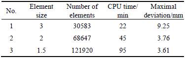
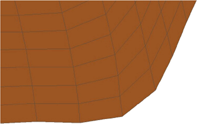
Fig. 12 About three elements around 90°bend obtained with mesh size of 1.5 mm
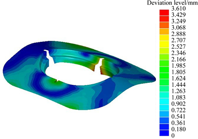
Fig. 13 Springback result
However, it is desirable to have the even smaller elements in the areas where the sharp bends are formed, but not on the large areas where a little deformation occurs. Fewer elements will reduce computation time and improve the convergence rate during the implicit springback simulation. In an attempt to obtain that, in the following, two methods will be applied, firstly, the adaptive mesh function will be utilized, secondly, a mesh with a variable mesh size will be constructed with the tools available in LS-Prepost.
The adaptive mesh function of Dynaform is utilized with an attempt to get small elements localized in areas with large deformation and larger elements in areas with little deformation. The hydroforming simulation is performed with an element size of 3 mm. Adaptive mesh is then activated for the subsequent rigid forming simulation, as seen in Fig. 14. This approach gives the desired situation of 4-5 elements around the final bends. However, the forming simulation is time-consuming, and the springback results are incoherent with other obtained results. Because of this, the adaptive mesh approach is abandoned.
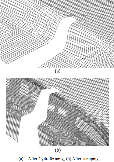
Fig. 14 Simulations with adaptive mesh
Blank with a custom mesh size is developed using the geometry and mesh tools in LS-Prepost. Again, it is desired to get a smaller mesh in the area with large deformation. The custom blanks before and after forming are seen in Figs. 15 and 16, respectively. The flange elements are roughly scaled at 5 mm, and the smaller elements are around 1 mm. The custom blank is proved to be stable and yields good results. The custom blank contains 75224 elements, which is less than that of simulation No. 3 from Table 3. Simulation time is roughly the same, and the custom blank needs a smaller timestep because of the smaller elements.
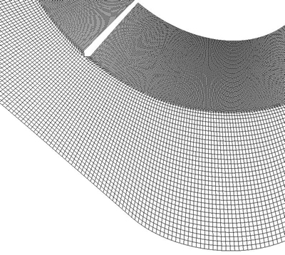
Fig. 15 Blank with a custom mesh before forming

Fig. 16 Blank with a custom mesh after forming
3.2 Influence of timesteps on springback model
It is possible to use two different approaches for the implicit springback analysis, single step springback or multiple step springback. Good results can be obtained with single step springback analysis, however, converged results might not be obtained using this approach for complex, flexible parts. It is therefore recommended to use multiple step springback analysis. Smaller timesteps should result in more accurate simulation results, but it will also increase time consumption.
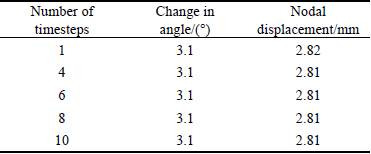
The results are listed in Table 4, along with the simulation time. Two different measurements are taken before and after springback for each timestep configuration, and then compared. A nodal displacement (point B) and an angle (angle A) are shown in Fig. 17. It is seen in Table 4 that there are no changes in the results of the last four timesteps. The only inconsistency is found in the nodal displacement for the single timestep analysis. Because of this, and the desire to get the shortest possible simulation time, four timesteps are found suitable for further usage.
Table 4 Results from springback analysis with different timesteps
3.3 Establishing springback model
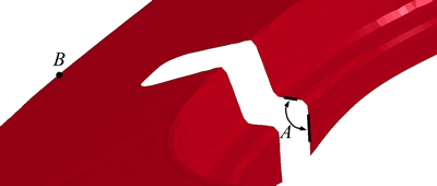
Fig. 17 Angle A and point B
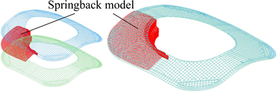
Fig. 18 Springback model with a quarter blank
The springback model can be seen in Fig. 18, with a quarter of a blank. Symmetry conditions are applied to the blank. The model is constrained with two surfaces defined as tools. This eliminates rigid body movement of the blank and allows for analysis of the springback behaviour in the critical areas only. The interpretation of these constrains are relevant in two scenarios, that forming is completed but the tools have not been opened yet, or that the part is mounted in the flange holes firstly and subsequently in the other three holes during assembly, as seen in Fig. 1. Also, according to the practical experiment, the springback is reduced for the process supplement part in the last step. Because of the sufficient deformation, the springback is not obvious after trimming. The part can meet the requirement of tolerances. The two tools are fully constrained rigid bodies. There is a gap of 1 mm between the tools, and the blank is positioned in the center of the gap. There is no gravity load applied. Mesh coarsening is not applied, because the performance of the model is good.
The springback simulation is static, so the implicit solver is used. The applied load in a springback simulation is determined from the initial stress in the sheet, which ceases to be in an equilibrium state after it is removed from the tools. The load must be applied slowly for complex springback simulation. In this simulation, the dieless method is adopted to resolve springback, the governing equation [21] is given as
 (1)
(1)
where Kn+1 is the stiffness matrix in the final forming timestep at n+1 moment; Δun+1 is the displacement increment at the n+1 moment;  is the nodal load force applied by the mould at the n+1 moment;
  is the nodal internal force at the n+1 moment and
  is the distributed contact force at the n+1 moment. When the is set to zero, the reverse solution is done for the force , which is exactly the dieless method. The flow chart [22] for the dieless springback simulation algorithm is shown in Fig. 19, where Ft is the contact stress of node at the last step of forming, and Fj is the equivalent nodal force.
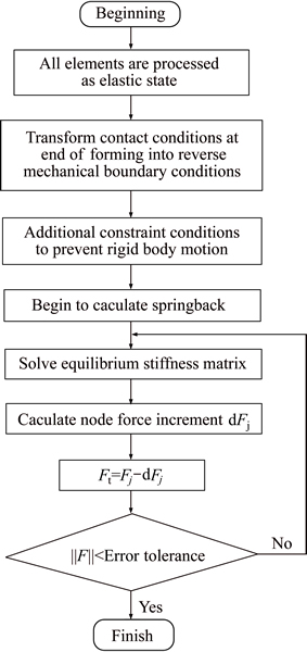
Fig. 19 Flow chart for dieless springback simulation algorithm
Different default values for the displacement and energy norms have been used so far. The parameters dctol and ectol in LS-Prepost choose two groups of different values, one is 0.001 and 1.0, and the other is 0.001 and 0.01, respectively. Next, the results of the springback model are evaluated, there will also be comparison of these two sets of values. The springback convergence criteria are based on displacement (dctol) and energy (ectol). Equilibrium iterations will cease when the result is close enough. The resulting nodal displacement for the different values of dctol and ectol is shown in Fig. 20.
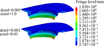
Fig. 20 Resulting nodal displacement for different values of dctol and ectol
The springback results will be validated by comparing the experimental data, it is found that angle θ3 will be a better metric. The location of the angle that will be compared is shown in Fig. 17. The springback value of angle θ3 is measured to be approximately 3.1°in the experiment, as seen in Fig. 21. Angle θ3 from the results seen in Fig. 20 is calculated to be approximately 3.3°. The results are satisfactory.

Fig. 21 Diagram of angle θ3
The results of the springback model have been validated. The model can now be used to investigate methods of reducing the springback behaviour of the part.
4 Strategy for reducing springback
For this part with complex geometry, the blank geometry has a great effect on the springback result of the part. Changing the blank geometry could be beneficial for reducing the springback. It is assumed that the four slips between the individual parts, as seen in Fig. 4, have been made to reduce the risk of fracture and meet the requirement of wall thickness reduction rate (only 10%), but because of these slips, there is almost uniaxial tension in the blank, when the bands are made. Figure 22 shows the major and minor engineering strain in plane, and the major strains are all almost perpendicular to the bend, while the minor strains are of a smaller magnitude, but negative. By changing the geometry of the blank, it is possible to change the strain and stress state in the blank after forming, and this will then affect the springback of the part.
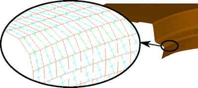
Fig. 22 Major and minor engineering strain in plane
Next, the genetic comparison methodology will be used for selection and developing blank geometries for development. This methodology is illustrated in Fig. 23. Initially, series of different 1st generation blank geometries is chosen. The series of simulations is performed and the springback result is compared to the result of a reference (the blank geometry is shown in Fig. 4). If the result is better than that of the reference, the blank geometry will be changed again and the new results will be evaluated. If the result is worse than that of the reference, the blank geometry is degraded. As shown in Fig. 23, the red indicates a springback result that is worse than that of the reference, and green indicates a springback result that is better than that of the reference.

Fig. 23 Illustration of methodology used for selection and developing blank geometries for development
Figure 24 shows the reference springback, with which the springback resulted from the different blank geometries (1st generation) will be compared. The green dotted line illustrates a result that is better than that of the reference. The red dotted line illustrates a result that is worse than that of the reference. Meanwhile, the springback of the part is compared with the reference at four different section planes, as illustrated in Fig. 25.
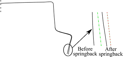
Fig. 24 Springback compared with reference
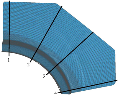
Fig. 25 Location of section planes
Some 1st generation blank geometries have been evaluated. The results of the springback simulations, with new blank geometries, have been compared with the reference. The results of comparison are shown in Fig. 26 (The black lines are references). The shapes of the two blanks can be seen in Fig. 27. In the red one, the slips have been removed, while leaving a local slip at the location of the third bend in the brown one. It is clear that the new blank geometries do not improve the results. The idea behind these two blank geometries is to create a more bi-axial tensile stress state, compared to that of the reference geometry.
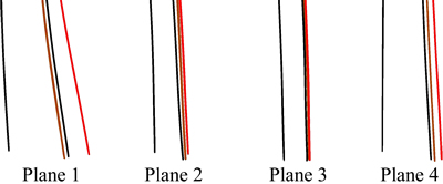
Fig. 26 Results of some of 1st generation compared with reference
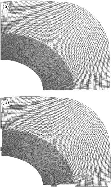
Fig. 27 Blank geometries that red one (a) and brown one (b) represent in Fig. 26
Figure 28 shows blank geometries with various degrees of success. In the first section cut, in Fig. 28, the golden blank shows more springback than that in the reference, but performs well when evaluated at the three other section cuts. The purple, yellow and green blanks show reduction of the springback in all the evaluated areas. The purple blank performs the best. The geometry of the purple blank is seen in Fig. 29(a).
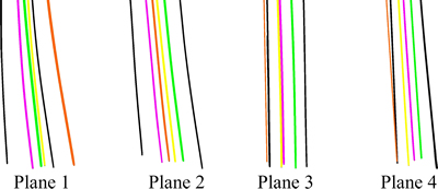
Fig. 28 Springback result for various blank geometries
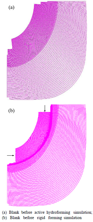
Fig. 29 Geometry of purple blank
After the active hydroforming simulation, additional elements are removed before the second rigid forming simulation. The blank before the second forming simulation is seen in Fig. 29(b), where the black arrows highlight the area where additional elements have been removed. From the four evaluation points, an average springback reduction of 58.8 % is estimated (as shown in Fig. 30).
In the experiments of the part with complex geometry, the springback is restrained effectively by using the purple blank shape. The final part is qualified and meets requirement of tolerances and assembling, as shown in Fig. 31.
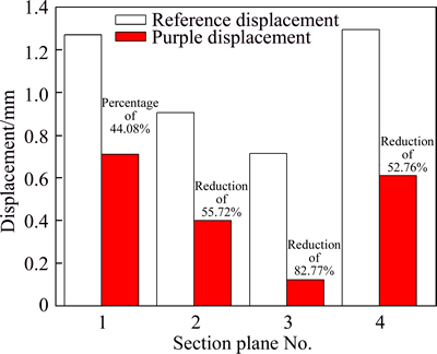
Fig. 30 Reduction of springback at four section cuts
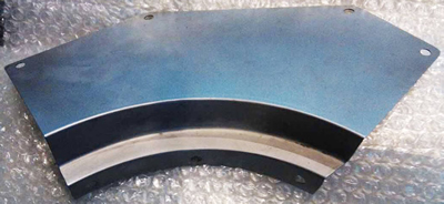
Fig. 31 Final part
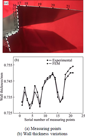
Fig. 32 Comparison of thickness distributions between experiments and FEM
The specimen thickness distribution is measured and compared with the result of the numerical simulation, as shown in Fig. 32. It can be seen that the wall thickness distribution of the whole specimen is uniform. The maximum thickness reduction rate is less than 10%. The experiment results coincide well with that of simulation.
5 Conclusions
1) The frictions between the tools and the blank, and between the dummy blank and the blank have a big effect on the stress in the sheet. The load path influences stress state through the thickness of the sheet in a relatively consistent way. And the binder force does not have a major influence on the results of the simulation.
2) The custom mesh size is beneficial for the springback simulation, compared with the constant mesh size and adaptive mesh size. Meanwhile, the four timesteps are found suited for the springback analysis for the complex geometry part.
3) The optimal blank geometry is obtained and used for manufacturing the part. Finally, the final obtained part is qualified and meets the requirement of tolerances and assembling.
References
[1] WAGONER R H, LI M. Simulation of springback: through-thickness integration [J]. International Journal of Plasticity, 2007,23(3): 345-360.
[2] LI Jian, ZHAO Jun, SUN Hong-lei, MA Rui. Improvement of springback prediction of wide sheet metal air bending process [J]. Journal of Central South University of Technology, 2010,15(S2): 310-315.
[3] CLEVELAND M, GHOSH A K. Inelastic effects on springback in metals [J]. International Journal of Plasticity, 2002,18(s5, 6): 769- 785.
[4] HAN Fei, MO Jian-hua, GONG Pan, LI Min. Method of closed loop springback compensation for incremental sheet forming process [J]. Journal of Central South University of Technology, 2011,18(5): 1509-1517.
[5] DAXIN E, LIU Y. Springback and time-dependent springback of 1Cr18Ni9Ti stainless steel tubes under bending [J]. Materials & Design,2010,31(3): 1256-1261.
[6] GENG L, WAGONER R H. Role of plastic anisotropy and its evolution on springback [J]. International Journal of Mechanical Sciences, 2002,44(1): 123-148.
[7] CHATTI S, HERMES M, WEINRICH A, BEN-KHALIFA N, TEKKAYA A E. New incremental methods for springback compensation by stress superposition [J]. International Journal of Material Forming,2009,2(1): 817-820.
[8] LINGBEEK R, HUETINK J, OHNIMUS S, PETZOLDT M, WEIHER J. The development of a finite elements based springback compensation tool for sheet metal products [J]. Journal of Materials Processing Technology,2005,169(1): 115-125.
[9] XIANG An-yang, FENG Ruan. A die design method for springback compensation based on displacement adjustment [J]. International Journal of Mechanical Sciences,2011,53(5): 399-406.
[10] WANG Hui, ZHOU Jie, ZHAO Tian-sheng, TAO Ya-ping. Springback compensation of automotive panel based on three-dimensional scanning and reverse engineering [J]. International Journal of Advanced Manufacturing Technology, 2015, 85(5): 1187- 1193.
[11] LEE J H, YOON J S, RYU C H, KIM S H. Springback compensation based on finite element for multipoint forming in shipbuilding [J]. Advanced Materials Research,2007,26-28: 981-984.
[12] PRETE A D, PRIMO T, STRANO M. The use of FEA packages in the simulation of a drawing operation with springback, in the presence of random uncertainty [J]. Finite Elements in Analysis & Design,2010,46(7): 527-534.
[13] LANG L H, JOACHIM D, KARL B N. Investigation into the effect of pre-bulging during hydromechanical deep drawing with uniform pressure onto the blank [J]. International Journal of Machine Tools & Manufacture, 2004, 44(6): 649-657.
[14] TAKAHASHI Y, IHARA T, KANAZAWA K. Fracture morphology accompanying fish-eye of austenitic stainless steel SUS321-B under long fatigue life region at 700 °C [J]. Transactions of Japan Society of Spring Engineers, 2014,2014(59): 19-28.
[15] TAKAHASHI Y, KOBAYASHI M, KANAZAWA K. Stepwise S-N curve and internal fracture of austenitic stainless steel under high temperature and high cycle fatigue conditions [J]. Journal of the Society of Materials Science Japan, 2013,62(2): 99-104.
[16] ASGARI A, PEREIRA M, ROLFE B, DINGLE M, HODGSON P. Design of experiments and springback prediction for AHSS automotive components with complex geometry [J]. Electronic Notes in Discrete Mathematics,2005,50(1, 2): 175-180.
[17] ANDERSSON A. Numerical and experimental evaluation of springback in advanced high strength steel [J]. Journal of Materials Engineering & Performance,2007,16(3): 301-307.
[18] SLOTA J, JURCISIN M. Experimental and numerical prediction of springback in V-bending of anisotropic sheet metals for automotive industry [J]. Journal of Applied Physiology,2012,84(3/12): 55-68.
[19] PAPADIA G, PRETE A D, ANGLANI A. Experimental springback evaluation in hydromechanical deep drawing (HDD) of large products [J]. Production Engineering,2012,6(2): 117-127.
[20] HARRISON D K, CHESHIRE D G, BAINES T S,
[21] ZHAO Dong-xu. The numerical simulation and technology optimization of the stamping forming of automotive lightweight steel and springback characteristics [D]. Changchun, China: Jilin University, 2007. (in Chinese)
[22] ZHANG Xiao-jing, ZHOU Xian-bin. Simulation of springback in sheet metal forming [J]. Journal of Plasticity Engineering, 1999, 6(3): 56-62. (in Chinese)
(Edited by FANG Jing-hua)
Cite this article as: WANG Yao, LANG Li-hui, S. Lauridsen, KAN Peng. Springback analysis and strategy for multi-stage thin-walled parts with complex geometries [J]. Journal of Central South University, 2017, 24(7): 1582-1593. DOI: 10.1007/s11771-017-3563-0.
Foundation item: Project(2014ZX04002041) supported by the National Science and Technology Major Project, China; Project(51175024) supported by the National Natural Science Foundation of China
Received date: 2016-04-06; Accepted date: 2016-07-11
Corresponding author: LANG Li-hui, Professor, PhD; Tel: +86-10-82316821; E-mail: lang@buaa.edu.cn

