Machine learning strategies for lithostratigraphic classification based on geochemical sampling data: A case study in area of Chahanwusu River, Qinghai Province, China
��Դ�ڿ������ϴ�ѧѧ��(Ӣ�İ�)2021���5��
�������ߣ������� ������ �ű�һ ����ܲ ��ΰϼ ������ Umair KHAN
����ҳ�룺1422 - 1447
Key words��machine learning; geochemical sampling; lithostratigraphic classification; lithostratigraphic prediction; bedrock
Abstract: Based on the complex correlation between the geochemical element distribution patterns at the surface and the types of bedrock and the powerful capabilities in capturing subtle of machine learning algorithms, four machine learning algorithms, namely, decision tree (DT), random forest (RF), XGBoost (XGB), and LightGBM (LGBM), were implemented for the lithostratigraphic classification and lithostratigraphic prediction of a quaternary coverage area based on stream sediment geochemical sampling data in the Chahanwusu River of Dulan County, Qinghai Province, China. The local Moran��s I to represent the features of spatial autocorrelations, and terrain factors to represent the features of surface geological processes, were calculated as additional features. The accuracy, precision, recall, and F1 scores were chosen as the evaluation indices and Voronoi diagrams were applied for visualization. The results indicate that XGB and LGBM models both performed well. They not only obtained relatively satisfactory classification performance but also predicted lithostratigraphic types of the Quaternary coverage area that are essentially consistent with their neighborhoods which have the known types. It is feasible to classify the lithostratigraphic types through the concentrations of geochemical elements in the sediments, and the XGB and LGBM algorithms are recommended for lithostratigraphic classification.
Cite this article as: ZHANG Bao-yi, LI Man-yi, LI Wei-xia, JIANG Zheng-wen, Umair KHAN, WANG Li-fang, WANG Fan-yun. Machine learning strategies for lithostratigraphic classification based on geochemical sampling data: A case study in area of Chahanwusu River, Qinghai Province, China [J]. Journal of Central South University, 2021, 28(5): 1422-1447. DOI: https://doi.org/10.1007/s11771-021-4707-9.

J. Cent. South Univ. (2021) 28: 1422-1447
DOI: https://doi.org/10.1007/s11771-021-4707-9

ZHANG Bao-yi(�ű�һ)1, 2, LI Man-yi(����ܲ)1, 2, LI Wei-xia(��ΰϼ)1, 2, JIANG Zheng-wen(������)1, 2,
Umair KHAN1, 2, WANG Li-fang(������)1, 2, WANG Fan-yun(������)1, 2
1. Key Laboratory of Metallogenic Prediction of Nonferrous Metals and Geological Environment Monitoring (Ministry of Education), Central South University, Changsha 410083, China;
2. School of Geosciences and Info-Physics, Central South University, Changsha 410083, China
 Central South University Press and Springer-Verlag GmbH Germany, part of Springer Nature 2021
Abstract: Based on the complex correlation between the geochemical element distribution patterns at the surface and the types of bedrock and the powerful capabilities in capturing subtle of machine learning algorithms, four machine learning algorithms, namely, decision tree (DT), random forest (RF), XGBoost (XGB), and LightGBM (LGBM), were implemented for the lithostratigraphic classification and lithostratigraphic prediction of a quaternary coverage area based on stream sediment geochemical sampling data in the Chahanwusu River of Dulan County, Qinghai Province, China. The local Moran��s I to represent the features of spatial autocorrelations, and terrain factors to represent the features of surface geological processes, were calculated as additional features. The accuracy, precision, recall, and F1 scores were chosen as the evaluation indices and Voronoi diagrams were applied for visualization. The results indicate that XGB and LGBM models both performed well. They not only obtained relatively satisfactory classification performance but also predicted lithostratigraphic types of the Quaternary coverage area that are essentially consistent with their neighborhoods which have the known types. It is feasible to classify the lithostratigraphic types through the concentrations of geochemical elements in the sediments, and the XGB and LGBM algorithms are recommended for lithostratigraphic classification.
Key words: machine learning; geochemical sampling; lithostratigraphic classification; lithostratigraphic prediction; bedrock
Cite this article as: ZHANG Bao-yi, LI Man-yi, LI Wei-xia, JIANG Zheng-wen, Umair KHAN, WANG Li-fang, WANG Fan-yun. Machine learning strategies for lithostratigraphic classification based on geochemical sampling data: A case study in area of Chahanwusu River, Qinghai Province, China [J]. Journal of Central South University, 2021, 28(5): 1422-1447. DOI: https://doi.org/10.1007/s11771-021-4707-9.
1 Introduction
With the advent of the era of big data, the ability to produce and store data far outpaces the ability to sensibly understand and assimilate them, and the paradigm of scientific research has accordingly changed. Under the fourth paradigm of big data thinking, the research object has changed from sampling data to overall data, and the goal of the research has shifted from pursuing causality to pursuing correlations [1]. We face two major tasks in the future: 1) extracting knowledge from the data deluge and 2) deriving models from the data that can learn much more than traditional approaches while still respecting our evolving understanding of nature��s laws [2]. Machine learning is a data analytical technique that teaches computers to learn information from data without being explicitly programmed [3].
Many of the leading approaches in machine learning are data-hungry, especially ��deep learning�� models [4]. Machine learning is often classified into unsupervised learning and supervised learning [5]. In supervised learning, both the input and the respective outputs are provided, and an algorithm aiming at building a nonlinear function to map new inputs to outputs by learning the relationship between input and output is proposed. In unsupervised learning, the algorithm does not have access to the output, so the goal of unsupervised learning is to infer the underlying structure of the data. Because of the ability to automatically extract patterns and knowledge from data, machine learning has been increasingly used to mine information from geospatial data and to solve geosciences problems, e.g., assessment and prediction of natural hazards [6, 7], environmental pollution monitoring [8, 9], and three-dimensional geological modeling [10, 11]. In mineral resource prediction, machine learning methods have been recommended for data-driven mineral prospectivity mapping where the number of occurrences is sufficient, and these methods are robust and effective regarding exploration target delineation [12-19]. Machine learning methods have also been used to identify geochemical patterns and to find anomalies that cannot be found by traditional methods; these methods focus on the correlation between the geological background and geochemical anomalies [20-25].
Lithostratigraphic classification, which aims to understand the distribution of subsurface lithology and formation, plays a vital role in geological research [26]. It is also an important basic work for mineral and hydrocarbon exploration. Traditional work involves regional geological mapping through outcrop observations to draw the distribution of different lithostratigraphic types. However, there are considerable limitations in areas with few outcrops. More accurate work involves obtaining rock samples through exploration engineering, e.g., trenches, wells, tunnels, and boreholes, or geophysical logging data [27]. Despite being time consuming and costly, this approach can only obtain the lithostratigraphic types of the bedrock within a limited area around the borehole, which makes it challenging to apply in a large area. To overcome these limitations, more attention has shifted towards intelligent machine learning techniques for automatic lithostratigraphic classification by using remote sensing data [28-30], well log data [31-35], geochemical sampling data [36, 37], and multivariate geosciences data [38, 39]. Lithostratigraphic classification based on remote sensing data essentially regards the whole study area as an image, and each training sample is a pixel, including spectrum information in the image. It is not trivial to integrate multi-sensor data since the image geometries, spatial and temporal resolution, physical meaning, content, and statistical data are different for different sensors [2]. In addition, due to the presence of clouds, vegetation or snow, lack of spectral information, and distortions in storage and transmission, the classification ability of classifiers based on remote sensing data is weakened. The geophysical well logging data are the measurements of physical properties of the rock in depth obtained from the borehole during, and after the drilling process using a variety of specialized instruments [40]. Geophysical well logging aims to obtain lithostratigraphic information in depth, and it is difficult to obtain training data in a large area.
A common characteristic of surface geochemical concentrations is that they are caused by upward migration of elements from the subsurface to the surface in various ways [41-44]. Mechanisms capable of transferring elements from the subsurface through barren transported cover to the surface are classified according to two main processes [45]: 1) phreatic processes, involving groundwater flow, convection, dilatancy, bubbles, diffusion and electromigration, and 2) vadose processes, involving capillary migration, gaseous transport and biological transfer. Therefore, lithostratigraphic classification can be conveniently performed in a large area using the geochemical concentrations sampled from the surface earth media, e.g., soil, stream sediment or lake sediment. Because of the migration of the elements from the subsurface to the surface during complex geological processes, the geochemical element distribution patterns at the surface are correlated to the types of bedrock in very complex way [46-48].
Machine learning methods have been proven powerful in capturing subtle, complex relationships between predictor and response variables. Some common supervised machine learning algorithms, such as support vector machine (SVM), decision tree (DT) and ensemble learning algorithms based on DT, have improved the accuracy and efficiency of lithostratigraphic classification. The SVM [49] achieves classification by constructing a decision surface that divides the instances into two parts in a high-dimensional feature space, which is a method for binary classification and has intrinsic limitations for the multiple classification. The DT [50] is the base classifier for many kinds of bagging and boosting ensemble learning algorithms. It can summarize rules from a series of data with features and labels to solve classification and regression problems, and presents these rules through a tree diagram structure. Because of its simple structure, it is not very computationally expensive. But when dealing with high-dimensional features or multiple classification tasks with too many types, the possibility of its misclassification will increase. KODIKARA et al [51] applied the DT classification method for lithological mapping from multispectral satellite imagery, and mapped accurate lithological variations in the vast rugged terrain. As DT cannot meet increasingly complex tasks, ensemble algorithms have developed. The efficiency of ensemble algorithms is usually better than that of a single DT because they combine the results of many decision tree classifiers. The random forest (RF) [52] is a typical bagging ensemble algorithm that combines tree predictors in parallel. Therefore, the efficiency of RF is usually better than that of a single DT in lithostratigraphic classification. HARRIS et al [38] produced meaningful predictive lithological maps of different rock types using RF classification. ORDONEZ-CALDERON et al [31] used different machine learning algorithms to predict different skarn types based on multielement geochemical data, and found that the predictive models yielded by the RF algorithm outperform those by all other algorithms. Boosting, another kind of ensemble learning algorithm, works by repeatedly running a given weak learning algorithm (such as DT) on various distributions over the training data, and then combining the classifiers produced by the weak learner into a single composite classifier [53]. Some typical boosting ensemble algorithms, e.g., AdaBoost [53], the gradient boosting decision tree (GDBT) [54], XGBoost (XGB) [55], and LightGBM (LGBM) [56], have exhibited surprisingly good performance in lithostratigraphic classification. JIANG et al [57] identified lithology based on mud logging data and wireline data using the boosting tree algorithm, and obtained a better correct rate than traditional methods, e.g., DT and SVM. DEV et al [32] evaluated recently developed boosting systems, e.g., XGB, LGBM and CatBoost, to classify formation lithology by using log data and found that LGBM produced the highest performance metrics. XIE et al [58] optimized the boosting method by regularization and stacking to further improve the accuracy of formation lithology classification compared with the single boosting method. ASANTE-OKYERE et al [59] exploited the advantage of incorporating results from clustering well log data using K-means and Gaussian mixture models (GMM) to construct a more accurate gradient-boosted machine (GBM) lithology model. In addition, deep learning methods have also been applied in rock mineral recognition under the microscope, which are essentially image recognition techniques that require much more labeled training data than ordinary machine learning as support [60-63].
Considering the high-dimensional features in lithostratigraphic classification, ensemble learning algorithms are more potential than a base leaner, DT. RF is a bagging ensemble algorithm to parallelly combine the results of many DT classifiers. XGBoost uses regularization and column sampling to reduce over-fitting. The highlight of LGBM is that it proposes gradient-based one-side sampling (GOSS), exclusive feature bundling (EFB) and leaf-wise strategies in order to save running time. Therefore, we chose different ensemble algorithms, random forest (RF), XGBoost (XGB) and LightGBM (LGBM), and compared them with their base learner, DT. The classification models using different supervised machine learning algorithms were trained with labeled geochemical sampling data according to the geological map of the study area. We calculated the local spatial autocorrelation coefficients of 15 geochemical elements, Moran��s I [64] within a distance of 1500 m, to represent the features of spatial autocorrelations. Moreover, we extracted three terrain factors, i.e., the elevation, slope and slope of aspect, to represent the features of surface geological processes as additional features. During model training, cross-validation, validation curves and grid search were implemented. We chose the accuracy, precision, recall, and F1 scores as the evaluation indices and visualized the results through Voronoi diagrams. Finally, we applied the classification models with XGB and LGBM algorithms to predict the types of bedrock under the Quaternary coverage area.
2 Methods
2.1 Decision tree
The DT is a tree structure (binary tree or multibranch tree) algorithm consisting of directed edges and nodes. Figure 1 shows a simple DT structure for dataset D with n classes. Leaves of a tree are class names, and other nodes represent attribute-based tests with a branch for each possible outcome. To classify an instance, the technique starts at the root node, selects one attribute for testing, evaluates the result, and passes through appropriate branches to one certain outcome. The process continues until leaf nodes are encountered, while the instance is asserted to belong to the class named by the leaf. Classification rules are therefore expressed as a DT.
The test attribute is crucial because the quality of a tree depends on the attribute-based test. There are different DT algorithms due to different evaluation functions. Commonly used algorithms are the iterative dichotomiser 3 (ID3) [50], C4.5 [65], and classification and regression tree (CART) [66].
The CART algorithm, applied in this paper, aims to find the best attribute-based test by the Gini impurity. The Gini impurity is used to measure the impurity of a dataset. The smaller the Gini impurity, the higher the purity of the dataset, i.e., the higher the probability that an instance in the dataset belongs to a certain class.
In practical solutions, the size of the dataset is usually large, and the corresponding tree is complicated and may involve some abnormal branches, so pruning is needed. If the internal nodes of a DT are {T1, T2, T3, ��, Tn}, the pruning strategy of CART is described as follows: 1) Calculate the surface error rate gain ��={��1, ��2, ��3, ��, ��n} for all internal nodes; 2) Select the internal node Ti with the smallest ��i (If there are several internal nodes with the same smallest ��i, the one with the most child nodes will be selected); and 3) Prune Ti. The surface error rate gain �� here is calculated as:
 (1)
(1)
where R(t) represents the error cost of the leaf nodes, R(T) represents the error cost of the subtree (the internal node with its child nodes), and N(T) represents the number of nodes of the subtree.

Figure 1 Structure of a DT (Xn represents test attributes, and Cn is a constant threshold representing the best attribute-based test)
A DT should not grow indefinitely. To stop growing in advance may help reduce the complexity of the tree structure and improve the performance of the prediction. There are several conditions for stopping: 1) When the number of samples on the node is less than a set threshold to weaken the role of noise; 2) When the Gini impurity of the node is less than a set threshold; 3) When the depth of the tree reaches a set threshold to reduce the complexity of the tree; and 4) When all attributes have been tested.
2.2 Random forest
The ensemble algorithm completes the classification or regression task by combining base learners. This approach reduces the variance or bias of the model and generally obtains better performance than the individual base learners. The RF [52] is a typical bagging ensemble algorithm. The bagging divides the dataset into several subsets, builds mutually independent models on each subset, and integrates the prediction results of these models. The RF combines several CART trees into a forest, and the final prediction is the mode (for classification task) or average (for regression task) of all trees. Figure 2 shows the flowchart of an RF with m trees, which can be described as follows: 1) Divide dataset D into m bootstrap subsets (i.e., sampling with replacement); 2) Generate m trees on m subsets, and subsample their features when generating trees; 3) Obtain m predictions by all trees; and 4) Calculate the mode or average of the m predictions as the final output.
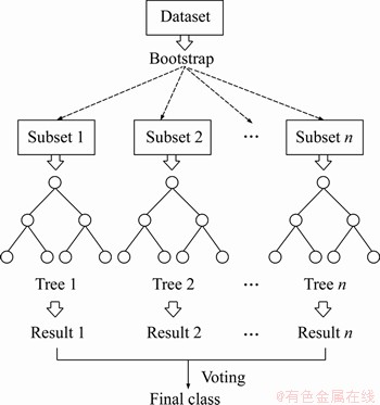
Figure 2 Flowchart of RF
2.3 XGBoost
XGB [55] is a highly scalable end-to-end tree boosting system that has been applied to various applications. The weak learner of XGB is the DT. When generating the trees, a weighted quantile sketch, instead of greedy algorithms, is proposed to select candidate split points, which increases efficiency for learning tasks with large-scale data. In addition, XGB incorporates a novel sparsity-aware algorithm to add a default direction in each tree node. The instance with a missing value in the sparse matrix will be classified into the default direction. Moreover, the sparsity-aware algorithm exploits the sparsity to make the computation complexity scale linearly with the number of non-missing instances. Similar to the RF, XGB also supports column (feature) subsampling, not only to reduce the computational cost but also to reduce the risk of overfitting. XGB uses additive functions to predict the output, taking the regression DT as the base learner.
To avoid overfitting, a regularization term ��(fk) is introduced into the objective function of XGB to control the complexity of the tree and reduce the impacts between trees through shrinkage. Let  be the prediction of the ith instance at the tth iteration. The goal is to minimize the regularized objective function:
 (2)
(2)
where  l is a differentiable convex loss function that measures the gap between the target yi
 and the prediction
  and �� is a penalty term for model complexity, which is used to help smooth the final learning weights and avoid overfitting.
When learning the tree structure, it is impossible to enumerate all the tree structures, so a greedy algorithm, which starts from the root node and adds branches to the tree iteratively from top to bottom according to a specific split basis, is usually used. Assuming that IL and IR are the instance sets of left and right nodes after the split, then the loss reduction after the split is given by:
 (3)
(3)
where Lsplit is usually used in practice for evaluating the split candidates. Here,  and
and  represent the scores of the left and right nodes after the split,
  represents the scores before the split, and �� represents the cost of complexity after splitting.
To reduce the computational costs, especially when memory is limited, an approximate algorithm is summarized in XGB. The algorithm first proposes candidate split points based on the percentiles of the feature distribution. Then, the continuous features are mapped into intervals split by these candidate points, and the statistics are accumulated to find the best split among the candidate splits.
2.4 Light GBM
Because XGB needs to scan the entire dataset at each iteration, the efficiency and scalability of XGB cannot meet the needs of studies with high-dimensional features, which is very time consuming. To solve this problem, KE et al [56] designed the LGBM algorithm. Compared with XGB, LGBM has shown amazing efficiency, accuracy and capabilities of big dataset processing. Its main innovations are two novel techniques, i.e., gradient-based one-side sampling (GOSS) and exclusive feature bundling (EFB).
Because an instance with a larger gradient plays a more important role in the computation of information gain, GOSS performs random sampling on the instances with small gradients and retains the instances with large gradients so that instances with a large gradient occupy the main positions in the information gain estimation. Such a treatment can lead to a more accurate gain estimation than indiscriminately random sampling. Specifically, the process of the GOSS is as follows: 1) Sort all instances according to the absolute values of their gradients; 2) Select the top a%instances to generate a subdataset L with a large gradient; 3) Randomly select b(1-a) % instances of the rest to generate a subdataset S with a small gradient; 4) Multiply the sub-dataset S by a weight coefficient  and then merge it with the sub-dataset L into a combined sub-dataset; 5) Use the combined sub-dataset to estimate a base learner; 6) Repeat the above steps until convergence or a certain iteration number.
The EFB technique is used to deal with high-dimensional sparse features by bundling mutually exclusive features, which never take nonzero values simultaneously, to reduce the dimensions. High-dimensional features are usually sparse, so the EFB technique can safely bundle exclusive features into a single feature. Therefore, model training can be accelerated without losing accuracy after reducing the dimensions.
The strategy of generating trees in LGBM is leaf-wise, which is different from XGB with a level-wise strategy. The level-wise strategy treats leaf nodes in the current layer indiscriminately. However, some leaf nodes have low split gains, which brings unnecessary computational costs. The leaf-wise strategy selects the leaf node with the largest gain among all leaf nodes in the current layer when splitting. Trees generated through the leaf-wise strategy often have higher accuracy than those generated through level-wise; however, it is easy to generate overly complex tree structures and to overfit when the size of the dataset is small. LGBM generally controls the depth of the tree to avoid overfitting.
3 Study area and data
The case study is situated in the area of the Chahanwusu River of Dulan County, Qinghai Province, China. It belongs to the eastern part of the East Kunlun tectonic belt in central Qinghai Province, and the exposed strata are mainly clastic rocks and volcanic rocks. Magmatic rocks in the area were developed mainly in the pre-Caledonian, Caledonian, Variscan and Indosinian ages, among which the Indosinian neutral and acid intrusive rocks and Triassic neutral and acid volcanic rocks were the main bodies. The area has complex geological structures and rich mineral resources and is an important metallogenic belt of precious metals, nonferrous metals and ferrous metals in China. Through a series of previous geological explorations and scientific research works, a large number of geological and geochemical data have been obtained. Figure 3 shows the regional geological map of the study area.
In this paper, 4959 stream sediment geochemical sampling points, at a scale of 1:50000 in the studied area, were collected from the Qinghai Geological Survey Institute. We obtained the concentrations of 15 geochemical elements at each sampling point: Au, Sn, Ag, As, Sb, Bi, Co, Cu, La, Pb, Zn, W, Mo, Nb and Cd. Because of the close relationship between the spatial distribution pattern of geochemical elements and the lithostratigraphic types, the 4955 sampling points were labeled with lithostratigraphic types according to the geological map (Figure 3) at the scale of 1:50000 in the study area, of which 849 sampling points (the gray points in Figure 4) were located in the Quaternary coverage area. Except for the sampling points in the Quaternary, 4106 points of the rest of the dataset were randomly split into a training dataset (accounting for 80%, the black points in Figure 4) and a testing dataset (accounting for 20%, the red points in Figure 4). All 4106 points are labeled into ten lithostratigraphic types: lower Proterozoic Baishahe Group (Pt1 b), upper Triassic Elashan Group (T3 e), Neogene Guide Group (NG), monzogranite (�Ǧ�), moyite (�Φ�), monzonitic granitic porphyry (�ЦǦ�), diorite (�Ħ�) and monzonitic quartz diorite (�Ǧ�o). According to the properties of the rocks, we merged the ten lithostratigraphic types into five general lithostratigraphic types: lower Proterozoic Baishahe Group (Pt1 b), upper Triassic Elashan Group (T3e), Neogene Guide Group (NG), granite (��) and diorite (��). The details and the number of points of each lithostratigraphic type are shown in Table 1.

Figure 3 Geological map of Chahanwusu River area of Dulan County, Qinghai Province, China
We analyzed the concentrations of the main mineralization elements in several bedrocks which are widely distributed in the studied area, and compared the mean concentration values of them with those of the corresponding stream sediments. For the two formations, the elements concentrations in the bedrocks and their corresponding stream sediments are very close, especially in the upper triassic Elashan group, where the two kinds of concentration curves almost coincide. The most widely distributed bedrocks in the studied area are granodiorite (�æ�), monzogranite (�Ǧ�) and monzonitic granitic porphyry (�ЦǦ�). As shown in Figure 5, the element concentrations curves of these bedrocks are basically consistent with those of their corresponding stream sediments. In addition, the curves of other bedrocks also show a strong correlation between the concentration in bedrocks and their corresponding stream sediments. The results indicated that stream sediments inherit the geochemical composition of underlying bedrocks. It is feasible to distinguish bedrock by the geochemical element concentrations of stream sediments.
Considering the autocorrelation of the concentration of geochemical elements, we calculated the local spatial autocorrelation coefficient Moran��s I [64] of the 15 geochemical elements. Because the sampling density is 5 or 6 sampling points per square kilometer in the study area and all concentration variograms have good spatial structures in range of about 1500 m, we set the range of 1500 m as the threshold of adjacency for spatial matrix when calculating the Moran��s I statistics. A Voronoi diagram was used to visualize the local Moran��s I of the 15 geochemical elements in the studied area (Figure 6). The local Moran��s I coefficient measures the degree of spatial autocorrelation between sampling points and their neighbors. It describes the spatial distribution pattern of geochemical elements into positive correlation (high-value aggregation or low-value aggregation), negative correlation (high-value and low-value cross-aggregation) and random distribution.
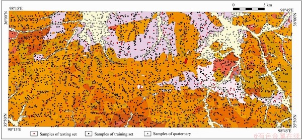
Figure 4 Spatial distribution of stream sediment geochemical sampling points, where black points are points in training dataset, red points are in testing dataset, and gray points are in Quaternary
Table 1 Lithostratigraphic types in studied area and number of sampling points

In addition, the terrain may cause the accumulation of geochemical elements in the stream sediments. Therefore, we extracted three terrain factors, i.e., the elevation (Figure 7(a)), slope (Figure 7(b)) and slope of aspect (Figure 7(c)), from the digital elevation model (DEM) of the studied area. The DEM data were downloaded from the geospatial data cloud (http://www.gscloud.cn/). The slope is calculated by the tangent value of the slope angle at the sampling points, which indicates how steep the surface is. The slope of the aspect refers to the change rate of the aspect. Based on the extracted aspect, the calculating principle of the slope is used to extract the change rate of the aspect. The calculation of the slope and the slope of the aspect involves the sampling point itself and its neighborhood, which considers the influence of the spatial neighborhood rather than treating the sampling point as an independent point in space.

Figure 5 Average concentrations of main mineralization elements in bedrocks, Lower Proterozoic Baishahe Group (Pt1b), Upper Triassic Elashan group (T3e), monzogranite (�Ǧ�), moyite (�Φ�), monzonitic granitic porphyry (�ЦǦ�), granodiorite (�æ�), granite quartz diorite (�æĦ�), and quartz diorite (�Ħ�), and their corresponding stream sediments (Blue curves describe mean values of element concentration in bedrocks during different geological periods, and red curves describe mean values of element concentration in their corresponding stream sediments)
4 Results
4.1 Model training
In this work, four different machine learning algorithms, i.e., the DT, RF, XGB and LGBM, were used to train different models. The concentrations of 15 geochemical elements and their respective local Moran��s I coefficients and three terrain factors of each sampling point were used as features to train models for the ten lithostratigraphic classifications and the five general lithostratigraphic classification tasks. We designed eight different classification models in total according to different tasks (Table 2).
To make the model predictive, part of the available training dataset is usually held out as a validation dataset when performing supervised machine learning. The complete processes of supervised machine learning usually include three stages: training the model on the training dataset, after which the model is evaluated on the validation dataset, and final evaluation on the testing dataset when obtaining the appropriate prediction model. The k-fold cross-validation with k=10 was used in this paper, which is a good solution to achieve this process and to avoid drastically reducing the number of sampling points. The k-fold cross-validation method randomly splits datasets into k sub-datasets, in which the identical distribution of each class is included. With these k sub-datasets, the training process is carried out on the k-1 sub-datasets, and the validation is carried out on the k-th sub-dataset. Each combination of parameters is evaluated k times, and the average is taken after k iterations. A good classifier should not only perform well during training; moreover, it should still perform well for unknown datasets. Therefore, for a well-trained classifier, the performance on a testing dataset, the remaining 20% of the whole dataset, is also used to evaluate its generalization.
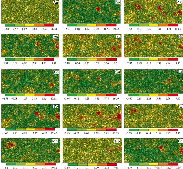
Figure 6 Voronoi diagrams of local Moran��s I coefficients for 15 geochemical elements in study area
The general process of machine learning is to use a model to fit a dataset and then to predict an unknown dataset using the trained model; therefore, a model with strong generalization is expected. However, there are often cases in which the generalization of the model is insufficient with underfitting or overfitting. The underfitting model has poor performance on both the training dataset and the testing dataset, while the overfitting model has extremely strong performance on the training dataset but has poor performance on the testing dataset because the noises of the training dataset are taken as features. To avoid overfitting, we tuned the parameters of the depth of the tree, the number of leaf nodes, and the number of trees to control the complexity of the models of the four tree-structure-based algorithms used in this paper.
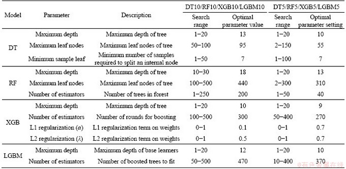
To improve the efficiency of the parameter tuning, we used validation curves after 10-fold cross-validation to set a range for parameter tuning and then determined the optimal parameters through the grid search. The validation curve is helpful to plot the influence of a single parameter on the training score and the validation score and to determine whether the model is overfitting or underfitting. If the cross-validation score increases with the training score, the model is underfitting. Conversely, if the training score increases with a decrease in the cross-validation score, the model is overfitting. Thus, the optimal parameters can be found through a grid search within the range where the training scores and the cross-validation scores do not change dramatically with the changes of the parameter values. The grid search generates candidates from a grid of parameter values and then evaluates all the possible combinations of parameter values to find the best combination. The validation curves of all models in this paper are shown in Figures 8-11. The search range and the optimal value of each parameter are shown in Table 3.

Figure 7 Images of elevation (a), slope (b) and slope of aspect (c) extracted from DEM
Table 2 Features and targets of different designed classification models

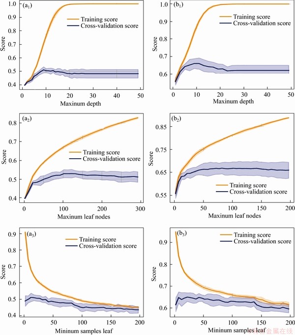
Figure 8 Validation curves of models DT10 (a) and DT5 (b)

Figure 9 Validation curves of models RF10 (a) and RF5 (b)
4.2 Evaluation metrics
The accuracy, precision, recall, and F1 scores were calculated with 10-fold cross-validation and used to evaluate the performances of the models in this work. The accuracy is the ratio of sampling points correctly classified by the classifier to the total number of points. The precision is the ratio of true predicted positive sampling points to the predicted positive points, whereas the recall is the percentage ratio of true predicted positive sampling points to the positive points. The F1 score is the harmonic mean of the precision and recall, which should be maximized as much as possible. All these metrics can be present in a confusion matrix, which also intuitively shows which class the instance is predicted as. The formulas are as follows:
 (4)
(4)
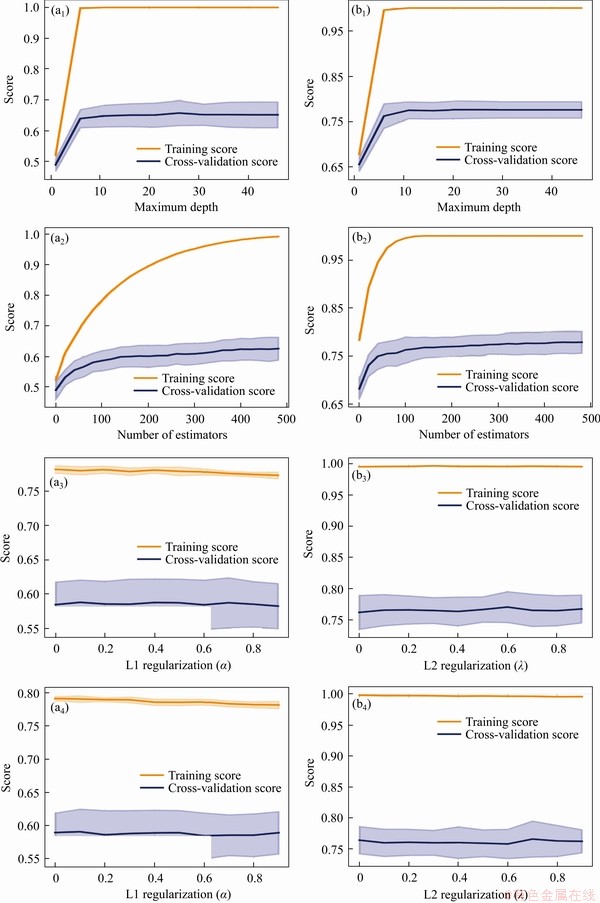
Figure 10 Validation curves of models XGB10 (a) and XGB5 (b)

Figure 11 Validation curves of models LGBM10 (a) and LGBM5 (b)
Table 3 Parameter tuning for models based on 10-fold cross-validation
 (5)
(5)
 (6)
(6)
 (7)
(7)
where TP is the number of true positive sampling points; TN is the number of true negative sampling points; FP is the number of false positive sampling points; FN is the number of false negative sampling points.
Voronoi diagrams were used to visualize the prediction results. A Voronoi diagram consists of a set of continuous sampling point centered polygons whose boundaries are the vertical bisectors of the lines of two adjacent points. This method is used to optimally segment two-dimensional space with a finite number of discrete points. Voronoi polygons associate each sampling point with its nearest neighbor. Therefore, it is reasonable to express the distribution of lithostratigraphic types throughout Voronoi diagrams.
4.3 Model performance
We trained eight different classification models towards different features and targets and chose accuracy, precision, recall and F1 score as the evaluation metrics.
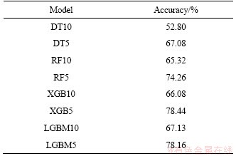
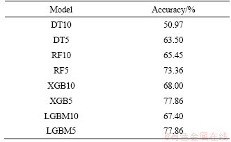
On the training dataset, the accuracies for the eight designed classification models are shown in Table 4. The algorithm with the best performance in the ten-type lithostratigraphic classification tasks is LGBM, with an accuracy of 67.13% after 10-fold cross-validation. The algorithm with the best performance in the generalized five-type lithostratigraphic classification tasks is XGB, with an accuracy of 78.44% after 10-fold cross-validation. Overall, the classification accuracy of RF, XGB and LGBM was higher than the accuracy of the DT; in particular, both XGB and LGBM performed surprisingly in our lithostratigraphic classification tasks.
Table 4 Accuracies of classification models on training dataset after 10-fold cross-validation
We present the confusion matrixes of the best performing algorithms XGB (Tables 5 and 6) and LGBM (Tables 7 and 8) in our two different classification tasks. In the ten-class lithostratigraphic classification, both precision and recall indices of the upper Triassic Elashan Group (T3e), granodiorite (�æ�) and monzonitic granitic porphyry (�ЦǦ�) were higher than others, that is, the geochemical elements in these bedrocks are more likely to migrate to their corresponding stream sediments; thus, higher F1 scores were obtained. In the generalized five-class lithostratigraphic classification, the precision of each class was high, especially that for granite. As shown in Table 9, the two different classification tasks, the classification accuracy on the testing dataset is significantly improved after merging the lithostratigraphic types. It is well understood that in the multiclassification problem, the more targets a learner needs to distinguish, the more difficult it is. In addition, after merging the lithostratigraphic types, the distributions of samples belonging to the same lithostratigraphic type are more concentrated and the spatial associations between samples become closer. Therefore, the accuracy of the generalized five-class lithostratigraphic classification is higher than that of the ten-class. However, it is worth noting that there is a great imbalance of our training dataset. There are far more sampling points labeled granite (��) and diorite (��) than other types, and only eight sampling points labeled Neogene guide group (NG), which causes high classification accuracy of the granite and diorite and incredibly low classification accuracy of the Neogene guide group. Most machine learning algorithms are based on the assumption that the training dataset is balanced; however, it is difficult to obtain a balanced dataset for training in practical geoscience problems. Therefore, how to solve the classification error caused by data imbalance requires attention.
Table 5 Confusion matrix for ten-type lithostratigraphic classification using XGB algorithm after 10-fold cross-validation

Table 6 Confusion matrix for generalized five-type lithostratigraphic classification using XGB algorithm after 10-fold cross-validation
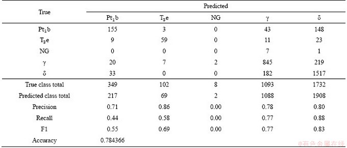
Table 7 Confusion matrix for ten-type lithostratigraphic classification using LGBM algorithm after 10-fold cross-validation
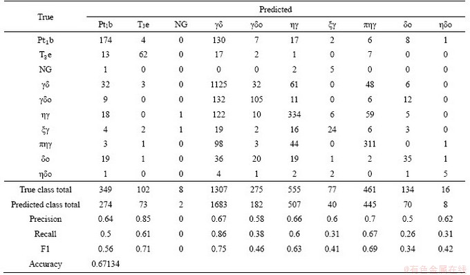
Table 8 Confusion matrix for generalized five-type lithostratigraphic classification using LGBM algorithm after 10-fold cross-validation

Table 9 Classification accuracy of each model on testing dataset
We compared the spatial distribution of lithostratigraphic classification with the geological map, and the Voronoi polygons of misclassification were marked (Figures 12 and 13). The classification performance was significantly higher on the generalized five-type lithostratigraphic classification than on the ten-type task. In all ten-type lithostratigraphic classification tasks, both XGB and LGBM predicted the lithostratigraphic distributions, which indicate major geological structures and trends. Although there are some scattered Voronoi polygons of misclassification, the spatial distributions of lithostratigraphic prediction substantially match the reference geological map. In summary, both XGB and LGBM have achieved better lithostratigraphic predictions than the other methods. The misclassification areas are mainly at the boundaries of different bedrocks, where the distributions of bedrocks are scattered and broken. On the other hand, the monzonitic quartz diorite (�Ǧ�o), quartz diorite (��o), moyite (�Φ�), and Neogene Guide Group (NG), which have a small number of samples in the studied area, are more likely to be misclassified. Machine learning algorithm as a kind of data-driven method, lacking of training samples will affect its performance.
4.4 Lithostratigraphic prediction under quaternary coverage
In the geological map, the areas marked as the Quaternary consist of sediments, where it is unable to determine the type of bedrock. In traditional works, it is necessary to adopt time-consuming and costly exploration methods to uncover sediments to extract underlying bedrock information.
Our work on the analysis of the labeled datasets suggests that our models can reliably classify lithostratigraphic types through geochemical sampling data. Therefore, to classify bedrock underlying the Quaternary sediments, we applied the trained classification models to predict the unlabeled lithostratigraphic types under the Quaternary sediments using the element concentrations of geochemical sampling points.
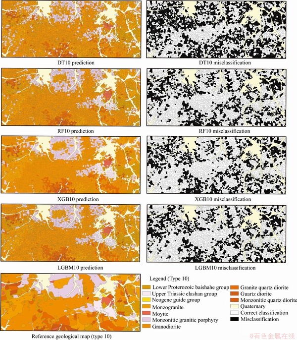
Figure 12 Spatial distribution of lithostratigraphic classification for ten-class lithostratigraphic classification
Because it is impossible to uncover all the Quaternary sediments to evaluate the predicted results quantitatively, we used a Voronoi diagram to map the predicted lithostratigraphic types of the Quaternary coverage. Figure 14 shows a Voronoi diagram of the Quaternary prediction using model XGB10. The actual lithostratigraphic types of neighboring areas of the Quaternary were retained, and three areas were selected for detailed display. The predicted types are essentially consistent with their neighbors that have the actual types, and the boundary lines of different lithostratigraphic types can be approximately distinguished according to the results.
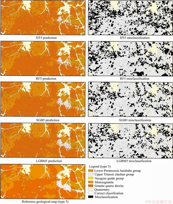
Figure 13 Spatial distribution of lithostratigraphic classification for generalized five-class lithostratigraphic classification (In addition to the dataset on the Quaternary coverage, the predicted lithostratigraphic type was gained, and the black polygons indicate the misclassification)
5 Discussion
In this study, we implemented the DT, RF, XGB and LGBM algorithms, all based on a tree structure, for the ten-type lithostratigraphic classification and the generalized five-type lithostratigraphic classification tasks. The cross-validation optimized the process of model selection to achieve the best performance in the testing dataset, which used part of the training dataset for training and the rest for validation. In this process, not only the training errors but also the prediction errors were considered. To improve the prediction ability and model performance of the model, it is necessary to adjust the hyperparameters of the model, e.g., the complexity of the tree and the number of trees. During hyperparameter tuning, the validation curves provided a reference for determining the tuning range, and the grid search effectively found the best combination of hyperparameters of each model.
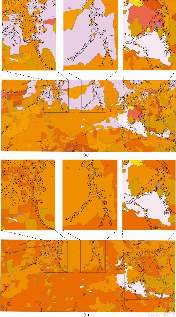
Figure 14 Spatial distribution of predicted bedrock types (refer to Figures 12 and 13 for detailed legend) underlying Quaternary by model XGB10 (a) and XGB5 (b) (Three areas were selected for detailed display on picture)
Of the four algorithms, the DT performs the worst and has neither adequate classification accuracy nor satisfactory spatial distribution predictions. The reason is that the simple structure of the DT makes it difficult for classification tasks with high-dimensional variables. In addition, the DT is a single learner, while the RF, XGB, and LGBM are ensemble learners, which combine predictions of all weak learners. The classification accuracy of the models using the RF, XGB, and LGBM are significantly higher than that of the DT. However, the visualization shows that distributions of lithostratigraphic classification with the XGB and LGBM are more consistent with the true lithostratigraphic distribution than that of the RF (Figure 12). Although the three algorithms are all ensemble learners, the RF is a parallel operation in which the weak learners are independent of each other. It can train weak learners at the same time, and then integrate their results through voting. However, XGB and LGBM are sequential operations in which the models are improved by constantly updating the weak learners. The weak learners in them must only be trained iteratively, which consumes more time than RF. Therefore, XGB and LGBM are more time-consuming than the RF, and their capabilities in mining the nonlinear correlation between features and targets are stronger than those of the RF.
As shown in the results (Figure 13), the predicted lithostratigraphic types of the Quaternary sampling dataset are essentially consistent with their neighbors that have the true types. This suggests that if a machine learning model can correctly classify the lithostratigraphic types, then it can be applied to the bedrock prediction of the Quaternary coverage in the study area. The distribution of the bedrock types underlying the Quaternary coverage can be obtained by machine learning. However, we cannot exactly know the true type of bedrock underlying the Quaternary coverage, so we can only evaluate the prediction results by Voronoi diagrams. We need to explore a quantitative analysis method based on spatial autocorrelation to evaluate the bedrock prediction results underlying the Quaternary coverage.
6 Conclusions
This work has achieved good performance in lithostratigraphic classification tasks and bedrock prediction underlying Quaternary coverage through models trained using the DT, RF, XGB and LGBM algorithms based on stream sediment geochemical sampling data. The implementation of cross-validation optimizes the process of model selection to achieve the best performance in the testing dataset. When hyperparameters tuning, the validation curves provide a reference for determining the tuning range, and the grid search effectively finds the best combination of hyperparameters of each model. Machine learning provides efficient approaches for data-driven lithological classification. Of the four algorithms, both XGB and LGBM perform satisfactorily with adequate classification accuracy and satisfactory spatial distribution predictions. Besides, we obtained the lithostratigraphic prediction underlying Quaternary coverage which is essentially consistent with their neighbors having the actual types and can approximately distinguish the boundary lines of different lithostratigraphic types. It is also found that the discriminate ability based on stream sediment geochemical data of different lithostratigraphic types exist diversities.
1) It is feasible to classify the lithostratigraphic types through the concentrations of geochemical elements in the sediments;
2) Machine learning can effectively improve the accuracy of lithostratigraphic classification, and the XGB and LGBM algorithms for lithostratigraphic classification are recommended;
3) If a machine learning model can correctly classify the lithostratigraphic types, then it can be applied to bedrock prediction underlying the Quaternary in the studied area.
Contributors
The overarching research goals were developed by ZHANG Bao-yi; WANG Li-fang provided the data curation and completed data preprocessing; LI Man-yi and LI Wei-xia trained the lithostratigraphic classifiers based on machine learning and predicted lithostratigraphic types underlying the Quaternary coverages; WANG Fun-yun analyzed and verified the results; JIANG Zheng-wen and Umair KHAN realized the visualization. The initial draft of the manuscript was written by ZHANG Bao-yi and LI Man-yi; WANG Li-fang replied to reviewers�� comments and revised the final version.
Conflict of interest
ZHANG Bao-yi, LI Man-yi, LI Wei-xia, JIANG Zheng-wen, Umair KHAN, WANG Li-fang, WANG Fan-yun declare that they have no conflict of interest.
Acknowledgments
The authors would like to thank the Co-Construction MapGIS Library by Engineering Research Center for Geographic Information System of China and Central South University for providing MapGIS software. We also thank senior engineer Professor ZHANG Shao-ning (The 8th Team of Qinghai Provincial Bureau of Nonferrous Metals and Geological Exploration) and Professor LAI Jian-qing (Central South University) for their kind assistance in the area of data collection.
References
[1] TOLLE K M, TANSLEY D S W, HEY A J G. the fourth paradigm: Data-intensive scientific discovery [J]. Proceedings of the IEEE, 2011, 99(8): 1334-1337. DOI: 10.1109/JPROC. 2011.2155130.
[2] REICHSTEIN M, CAMPS-VALLS G, STEVENS B, JUNG M, DENZLER J, CARVALHAIS N, PRABHAT. Deep learning and process understanding for data-driven earth system science [J]. Nature, 2019, 566(7743): 195-204. DOI: 10.1038/s41586-019-0912-1.
[3] BISHOP C M. Pattern recognition and machine learning [M]. Springer, 2007. https://www.springer.com/us/book/9780387 310732.
[4] LAKE B M, SALAKHUTDINOV R, TENENBAUM J B. Human-level concept learning through probabilistic program induction [J]. Science, 2015, 350(6266): 1332-1338. DOI: 10.1126/science. aab3050.
[5] MOHRI M, ROSTAMIZADEH A, TALWALKAR A. Foundations of machine learning [M]. MIT Press, 2018. https://ieeexplore.ieee.org/document/6282245?reload=true&tp= &arnumber=6282245.
[6] DEVRIES P M R, VIEGAS F, WATTENBERG M, MEADE B J. Deep learning of aftershock patterns following large earthquakes [J]. Nature, 2018, 560(7720): 632-634. DOI: 10.1038/s41586-018-0438-y.
[7] RAHMATI O, GOLKARIAN A, BIGGS T, KEESSTRA S, MOHAMMADI F, DALIAKOPOULOS I N. Land subsidence hazard modeling: Machine learning to identify predictors and the role of human activities [J]. J Environ Manage, 2019, 236: 466-480. DOI: 10.1016/j.jenvman. 2019.02.020.
[8] LI Tong-wen, SHEN Huan-feng, YUAN Qiang-qiang, ZHANG Xue-chen, ZHANG Liang-pei. Estimating ground-level PM2.5 by fusing satellite and station observations: A geo-intelligent deep learning approach [J]. Geophysical Research Letters, 2017, 44(23): 985-993. DOI: 10.1002/2017gl075710.
[9] WANG Rao, LI Qing-yong, YU Hao-min, CHEN Ze-chuan, ZHANG Ying-jun, ZHANG Ling, CUI Hou-xin, ZHANG Ke. A category-based calibration approach with fault tolerance for air monitoring sensors [J]. IEEE Sensors Journal, 2020, 20(18): 10756-10765. DOI: 10.1109/jsen.2020.2994645.
[10] ADELI A, EMERY X, DOWD P. Geological modelling and validation of geological interpretations via simulation and classification of quantitative covariates [J]. Minerals, 2017, 8(7): 8010007. DOI: 10.3390/min8010007.
[11] GONCALVES I G, KUMAIRA S, GUADAGNIN F. A machine learning approach to the potential-field method for implicit modeling of geological structures [J]. Computers and Geosciences, 2017, 103: 173-182. DOI: 10.1016/j.cageo. 2017.03. 015.
[12] MCKAY G, HARRIS J R. Comparison of the data-driven random forests model and a knowledge-driven method for mineral prospectivity mapping: A case study for gold deposits around the Huritz group and Nueltin suite, Nunavut, Canada [J]. Natural Resources Research, 2015, 25(2): 125-143. DOI: 10.1007/s11053-015-9274-z.
[13] RODRIGUEZ-GALIANO V, SANCHEZ-CASTILLO M, CHICA-OLMO M, CHICA-RIVAS M. Machine learning predictive models for mineral prospectivity: An evaluation of neural networks, random forest, regression trees and support vector machines [J]. Ore Geology Reviews, 2015, 71: 804-818. DOI: 10.1016/j.oregeorev.2015.01.001.
[14] CHEN Yong-liang, WU Wei. Isolation forest as an alternative data-driven mineral prospectivity mapping method with a higher data-processing efficiency [J]. Natural Resources Research, 2018, 28(1): 31-46. DOI: 10.1007/s11053-018-9375-6.
[15] ZHANG Nan-nan, ZHOU Ke-fa, LI Dong. Back-propagation neural network and support vector machines for gold mineral prospectivity mapping in the Hatu region, Xinjiang, China [J]. Earth Science Informatics, 2018, 11(4): 553-566. DOI: 10.1007/ s12145-018-0346-6.
[16] SUN Tao, CHEN Fei, ZHONG Lian-xiang, LIU Wei-ming, WANG Yun. GIS-based mineral prospectivity mapping using machine learning methods: A case study from tongling ore district, eastern China [J]. Ore Geology Reviews, 2019, 109: 26-49. DOI: 10.1016/j.oregeorev.2019. 04.003.
[17] KEYKHAY-HOSSEINPOOR M, KOHSARY A H, HOSSEIN-MORSHEDY A, PORWAL A. A machine learning-based approach to exploration targeting of porphyry Cu-Au deposits in the Dehsalm district, eastern Iran [J]. Ore Geology Reviews, 2020, 116: 103234. DOI: 10.1016/ j.oregeorev.2019. 103234.
[18] SUN Tao, LI Hui, WU Kai-xing, CHEN Fei, ZHU Zhong, HU Zi-juan. Data-driven predictive modelling of mineral prospectivity using machine learning and deep learning methods: A case study from southern Jiangxi province, China [J]. Minerals, 2020, 10(2): 10020102. DOI: 10.3390/ min10020102.
[19] WANG Fan-yun, MAO Xian-cheng, DENG Hao, ZHANG Bao-yi. Manganese potential mapping in western Guangxi-southeastern Yunnan (China) via spatial analysis and modal-adaptive prospectivity modeling [J]. Transactions of Nonferrous Metals Society of China, 2020, 30(4): 1058-1070. DOI: 10.1016/s1003-6326(20)65277-3.
[20] ZUO Ren-guang, XIONG Yi-hui. Big data analytics of identifying geochemical anomalies supported by machine learning methods [J]. Natural Resources Research, 2017, 27(1): 5-13. DOI: 10.1007/s11053-017-9357-0.
[21] CHEN Yong-liang, WU Wei. Application of one-class support vector machine to quickly identify multivariate anomalies from geochemical exploration data [J]. Geochemistry: Exploration, Environment, Analysis, 2017, 17(3): 231-238. DOI: 10.1144/geochem2016-024.
[22] CHEN Li-rong, GUAN Qing-feng, FENG Bin, YUE Han-qiu, WANG Jun-yi, ZHANG Fan. A multi-convolutional autoencoder approach to multivariate geochemical anomaly recognition [J]. Minerals, 2019, 9(5): 9050270. DOI: 10.3390/min9050270.
[23] WANG Zi-ye, ZUO Ren-guang, DONG Yan-ni. Mapping geochemical anomalies through integrating random forest and metric learning methods [J]. Natural Resources Research, 2019, 28(4): 1285-1298. DOI: 10.1007/s11053-019-09471-y.
[24] GHEZELBASH R, MAGHSOUDI A, CARRANZA E J M. Optimization of geochemical anomaly detection using a novel genetic K-means clustering (GKMC) algorithm [J]. Computers and Geosciences, 2020, 134: 104335. DOI: 10.1016/j.cageo. 2019.104335.
[25] WU Ruo-yu, CHEN Jian-li, ZHAO Jiang-nan, CHEN Jin-duo, CHEN Shou-yu. Identifying geochemical anomalies associated with gold mineralization using factor analysis and spectrum�Carea multifractal model in Laowan district, Qinling-Dabie metallogenic belt, central China [J]. Minerals, 2020, 10(3): 10030229. DOI: 10.3390/min10030229.
[26] GUO Zhen-wei, LAI Jian-qing, ZHANG Ke-ning, MAO Xian-cheng, LIU Jian-xin. Geosciences in central south university: A state-of-the-art review [J]. Journal of Central South University, 2020, 27(4): 975-996. DOI: 10.1007/ s11771-020-4347-5.
[27] SUN Jian, LI Qi, CHEN Ming-qiang, REN Long, HUANG Gui-hua, LI Chen-yang, ZHANG Zi-xuan. Optimization of models for a rapid identification of lithology while drilling-A win-win strategy based on machine learning [J]. Journal of Petroleum Science and Engineering, 2019, 176: 321-341. DOI: 10.1016/j.petrol.2019.01.006.
[28] YU Le, PORWAL A, HOLDEN E J, DENTITH M C. Towards automatic lithological classification from remote sensing data using support vector machines [J]. Computers and Geosciences, 2012, 45: 229-239. DOI: 10.1016/j.cageo.2011. 11. 019.
[29] PARAKH K, THAKUR S, CHUDASAMA B, TIRODKAR S, BHATTACHARYA A. Machine learning and spectral techniques for lithological classification [C]// SPIE Asia-Pacific Remote Sensing, 2016: 1-12. DOI: 10.1117/ 12.2223638.
[30] CRACKNELL M J, READING A M. Geological mapping using remote sensing data: A comparison of five machine learning algorithms, their response to variations in the spatial distribution of training data and the use of explicit spatial information [J]. Computers and Geosciences, 2014, 63: 22-33. DOI: 10.1016/j.cageo.2013.10.008.
[31] ORDONEZ-CALDERON J C, GELCICH S. Machine learning strategies for classification and prediction of alteration facies: Examples from the Rosemont Cu-Mo-Ag skarn deposit, SE Tucson Arizona [J]. Journal of Geochemical Exploration, 2018, 194: 167-188. DOI: 10.1016/j.gexplo. 2018.07.020.
[32] DEV A D, EDEN M R. Formation lithology classification using scalable gradient boosted decision trees [J]. Computers and Chemical Engineering, 2019, 128: 392-404. DOI: 10.1038/s41586-018-0438-y.
[33] KITZIG M, KEPIC A, GRANT A. Near real-time classification of iron ore lithology by applying fuzzy inference systems to petrophysical downhole data [J]. Minerals, 2018, 8(7): 8070276. DOI: 10.3390/min 8070276.
[34] XIE Yun-xin, ZHU Chen-yang, ZHOU Wen, LI Zhong-dong, LIU Xuan, TU Mei. Evaluation of machine learning methods for formation lithology identification: A comparison of tuning processes and model performances [J]. Journal of Petroleum Science and Engineering, 2018, 160: 182-193. DOI: 10.1016/j.petrol.2017.10.028.
[35] SUN Jian, LI Qi, CHEN Ming-qiang, REN Long, HUANG Gui-hua, LI Chen-yang, ZHANG Zi-xuan. Optimization of models for a rapid identification of lithology while drilling-A win-win strategy based on machine learning [J]. Journal of Petroleum Science and Engineering, 2019, 176: 321-341. DOI: 10.1016/j.petrol.2019.01.006.
[36] SAVU-KROHN C, RANTITSCH G, AUER P, MELCHER F, GRAUPNER T. Geochemical fingerprinting of Coltan ores by machine learning on Uneven datasets [J]. Natural Resources Research, 2011, 20(3): 177-191. DOI: 10.1007/s11053-011-9142-4.
[37] CATE A, SCHETSELAAR E, MERCIER-LANGEVIN P, ROSS P-S. Classification of lithostratigraphic and alteration units from drillhole lithogeochemical data using machine learning: A case study from the Lalor volcanogenic massive sulphide deposit, Snow Lake, Manitoba, Canada [J]. Journal of Geochemical Exploration, 2018, 188: 216-228. DOI: 10.1016/j.gexplo.2018.01. 019.
[38] HARRIS J R, GRUNSKY E C. Predictive lithological mapping of Canada��s north using random forest classification applied to geophysical and geochemical data [J]. Computers and Geosciences, 2015, 80: 9-25. DOI: 10.1016/ j.cageo.2015. 03.013.
[39] COSTA I, TAVARES F, OLIVEIRA J. Predictive lithological mapping through machine learning methods: A case study in the Cinzento Lineament, Caraj��s province, Brazil [J]. Journal of the Geological Survey of Brazil, 2019, 2(1): 26-36. DOI: 10.29396/jgsb.2019.v2.n1.3
[40] ELLIS D V, SINGER J M. Well logging for earth scientists [M]. Netherlands: Springer, 2007. DOI: 10.1007/978-1-4020-4602-5.
[41] CHENG Qiu-ming. Singularity theory and methods for mapping geochemical anomalies caused by buried sources and for predicting undiscovered mineral deposits in covered areas [J]. Journal of Geochemical Exploration, 2012, 122: 55-70. DOI: 10.1016/j.gexplo.2012.07.007.
[42] SHAHI H, GHAVAMI R, ROUHANI A K. Detection of deep and blind mineral deposits using new proposed frequency coefficients method in frequency domain of geochemical data [J]. Journal of Geochemical Exploration, 2016, 162: 29-39. DOI: 10.1016/j.gexplo.2015.12.006.
[43] CHEN Qiao, JIA Cui-ping, WEI Jiu-chuan, DONG Fan-ying, YANG Wei-gang, HAO De-cheng, JIA Zhi-wei, JI Yu-han. Geochemical process of groundwater fluoride evolution along global coastal plains: Evidence from the comparison in seawater intrusion area and soil salinization area [J]. Chemical Geology, 2020, 552: 119779. DOI: 10.1016/ j.chemgeo.2020.119779.
[44] CHEN Qiao, HAO De-cheng, WEI Jiu-chuan, JIA Cui-ping, WANG Hong-mei, SHI Long-qing, LIU Song-liang, NING Fang-zhu, AN Mao-guo, JIA Zhi-wei, DONG Fang-ying, JI Yu-han. The influence of high-fluorine groundwater on surface soil fluorine levels and their FTIR characteristics [J]. Arabian Journal of Geosciences, 2020, 13: No. 383. DOI: 10.1007/s12517-020-05346-2.
[45] ANAND R R, ASPANDIAR M F, NOBLE R R P. A review of metal transfer mechanisms through transported cover with emphasis on the vadose zone within the Australian regolith [J]. Ore Geology Reviews, 2016, 73(3): 394-416. DOI: 10.1016/j. oregeorev.2015.06.018.
[46] ZAREMOTLAGH S, HEZARKHANI A. The use of decision tree induction and artificial neural networks for recognizing the geochemical distribution patterns of LREE in the Choghart deposit, central Iran [J]. Journal of African Earth Sciences, 2016, 128: 37-46. DOI: 10.1016/j.jafrearsci.2016. 08.018.
[47] ZHANG Bao-yi, CHEN Yi-ru, HUANG An-shuo, LU Hao, CHENG Qiu-ming. Geochemical field and its roles on the 3D prediction fo concealed ore-bodies [J]. Acta Petrologica Sinica, 2018, 34(2): 352-362. http://en.cnki.com.cn/Article_en/ CJFDTotal-YSXB201802012.htm. (in Chinese)
[48] WANG Li-fang, WU Xiang-bin, ZHANG Bao-yi, LI Xue-feng, HUANG An-shuo, MENG Fei, DAI Peng-yao. Recognition of significant surface soil geochemical anomalies via weighted 3d shortest-distance field of subsurface orebodies: A case study in the Hongtoushan copper mine, NE China [J]. Natural Resources Research, 2019, 28(3): 587-607. DOI: 10.1007/s11053-018-9410-7.
[49] CORTES C, VAPNIK V. Support-vector networks [J]. Machine Learning, 1995, 20(3): 273-297. DOI: 10.1023/A:1022627411411.
[50] QUINLAN J R. Induction of decision trees [J]. Machine Learning, 1986, 1(1): 81-106. DOI: 10.1023/ A:1022643204877.
[51] KODIKARA J R L, WOLDAI T. Spectral indices derived, non-parametric decision tree classification approach to lithological mapping in the Lake Magadi area, Kenya [J]. International Journal of Digital Earth, 2017, 11(10): 1020-1038. DOI: 10.1080/17538947. 2017.1372525.
[52] BREIMAN L. Random forests [J]. Machine Learning, 2001, 45(1): 5-32. DOI: 10.1023/A:1010933404324.
[53] FREUND Y, SCHAPIRE R E. Experiments with a new boosting algorithm [C]// International Conference on Machine Learning: Proceedings of the Thirteenth International Conference. 1996: 148-156. http://cseweb. ucsd.edu/~yfreund/papers/boostingexperiments.pdf.
[54] FRIEDMAN J H. Stochastic gradient boosting [J]. Computational Statistics & Data Analysis, 2002, 38(4): 367-378. DOI: 10.1016/S0167-9473(01)00065-2.
[55] CHEN Tian-qi, GUESTRIN C. XGBoost: A scalable tree boosting system [C]// the 22nd ACM SIGKDD International Conference on Knowledge Discovery and Data Mining. San Francisco, California, USA: Association for Computing Machinery, 2016: 785-794. DOI: 10.1145/2939672.2939785.
[56] KE Guo-lin, MENG Qi, FINLEY T, WANG Tai-feng, CHEN Wei, MA Wei-dong, YE Qi-wei, LIU Tie-Yan. LightGBM: A highly efficient gradient boosting decision tree [C]// Neural Information Processing Systems 30 (NIPS 2017). Long Beach, CA, USA: Neural Information Processing Systems Conference, 2017: 3149-3157. http://papers.nips.cc/paper/ 6907-lightgbm-a-highly-efficient-gradient-boosting-decision -tree.pdf.
[57] JIANG Kai, WANG Shou-dong, HU Yong-jing, PU Shi-zhao, DUAN Hang, WANG Zheng-wen. Lithology identification model by well logging based on boosting tree algorithm [J]. Well Logging Technology, 2018, 42(4): 29-34. http://en.cnki.com.cn/Article_en/CJFDTotal-CJJS20180400 6.htm. (in Chinese)
[58] XIE Zheng-wen, ZHU Chen-yang, LU Yue, ZHU Zheng-wei. Towards optimization of boosting models for formation lithology identification [J]. Mathematical Problems in Engineering, 2019, 5309852. DOI: 10.1155/2019/5309852.
[59] ASANTE-OKYERE S, SHEN Chuan-bo, ZIGGAH Y Y, RULEGEYA M M, ZHU Xiang-feng. A novel hybrid technique of integrating gradient-boosted machine and clustering algorithms for lithology classification [J]. Natural Resources Research, 2019, 29(4): 2257-2273. DOI: 10.1007/s11053-019-09576-4.
[60] GOODFELLOWI J, POUGET-ABADIE J, MIRZA M, XU Bing, WARDE-FARLEY D, OZAIR S, COURVILLE A, BENGIO Y. Generative adversarial networks [C]// Advances in Neural Information Processing Systems. Montr��al, Canada: 2014: 2672-2680. https://arxiv.org/pdf/1406.2661v1.pdf.
[61] XU Shu-teng, ZHOU Yong-zhang. Artificial intelligence identification of ore minerals under microscope based on deep learning algorithm [J]. Acta Petrologica Sinica, 2018, 34(11): 3244-3252. http://html.rhhz.net/ysxb/20181110.htm. (in Chinese)
[62] LI Guo-he, QIAO Ying-han, ZHENG Yi-feng, LI Ying, WU Wei-jiang. Semi-supervised learning based on generative adversarial network and its applied to lithology recognition [J]. IEEE Access, 2019, 7: 67428-67437. DOI: 10.1109/access. 2019.2918366.
[63] LIU Cheng-zhao, LI Ming-chao, ZHANG Ye, HAN Shuai, ZHU Yue-qin. An enhanced rock mineral recognition method integrating a deep learning model and clustering algorithm [J]. Minerals, 2019, 9: 516. DOI: 10.3390/min9090516.
[64] ANSELIN L. Local indicators of spatial association��LISA [J]. Geographical Analysis, 1995, 27(2): 93-115. DOI: 10.1111/j.1538-4632.1995.tb 00338.x.
[65] QUINLAN J R. C4.5 : Programs for machine learning [M]. San Francisco: Morgan Kaufmann Publishers Inc, 1993. DOI: 10.5555/152181.
[66] BREIMAN L, FRIEDMAN J, OLSHEN R A, STONE C J. Classification and regression trees [M]. New York: Chapman and Hall, 1984. DOI: 10.2307/2530946.
(Edited by FANG Jing-hua)
���ĵ���
���ڻ���ѧϰ�ĵ���ѧ�����·����������б����ຣʡ�캹���պӵ���Ϊ��
ժҪ���������͵��б��ǵ��ʵ�����ʮ����Ҫ�����ݣ�Ҳ�ǿ�չ������̽�Ϳ����̽����Ҫ�������������IJ��þ����������ɭ�֡�XGBoost��LightGBM���ֻ���ѧϰ�ķ�����ʵ���˻��ڵ���ѧ�������ݵĻ��������б���15�ֵ���ѧԪ�غ�������ֲ��ռ������Ī��ָ���͵�������Ϊ������ѵ���˲�ͬ�ķ���ģ�ͣ�ͨ��10�۽�����֤��ģ����������֤�����ۡ��������������ѧϰ�㷨�ķ���Ч�����ھ�����������XGBoost��LightGBM������ã��Ը��ӵĸ�ά�ռ����ݺͲ�ƽ�������н�ǿ�Ĵ������������⣬����ͨ�������ķ���ģ�ͳɹ���ʵ���˶Ե���ϵ�������·��������͵�Ԥ�⣬ Voronoiͼ���ӻ����������Ԥ���������������Χ��ʵ�������ͻ����Ǻϣ��ܳ��������������͵ķֽ��ߡ���ˣ����õ���ѧ�����������б����·����������ǿ��еġ�
�ؼ��ʣ�����ѧϰ������ѧ���������������б𣻵���ϵ�·���������Ԥ��
Foundation item: Projects(41772348, 42072326) supported by the National Natural Science Foundation of China; Project(2017YFC0601503) supported by the National Key Research and Development Program, China
Received date: 2020-05-23; Accepted date: 2020-09-20
Corresponding author: WANG Li-fang, PhD, Engineer; Tel: +86-731-88877676; E-mail: csuwlf@139.com; ORCID: https://orcid.org/ 0000-0001-8950-4069; WANG Fan-yun, PhD; Tel: +86-731-88877676; E-mail: wfy8397641@163.com; ORCID: https://orcid.org/0000-0002-1118-1906

