Linear manifold clustering for high dimensional data based online manifold searching and fusing
来源期刊:中南大学学报(英文版)2010年第5期
论文作者:黎刚果 王正志 王晓敏 倪青山 强波
文章页码:1058 - 1069
Key words:linear manifold; subspace clustering; line manifold; data mining; data fusing; clustering algorithm
Abstract: High dimensional data clustering, with the inherent sparsity of data and the existence of noise, is a serious challenge for clustering algorithms. A new linear manifold clustering method was proposed to address this problem. The basic idea was to search the line manifold clusters hidden in datasets, and then fuse some of the line manifold clusters to construct higher dimensional manifold clusters. The orthogonal distance and the tangent distance were considered together as the linear manifold distance metrics. Spatial neighbor information was fully utilized to construct the original line manifold and optimize line manifolds during the line manifold cluster searching procedure. The results obtained from experiments over real and synthetic data sets demonstrate the superiority of the proposed method over some competing clustering methods in terms of accuracy and computation time. The proposed method is able to obtain high clustering accuracy for various data sets with different sizes, manifold dimensions and noise ratios, which confirms the anti-noise capability and high clustering accuracy of the proposed method for high dimensional data.
J. Cent. South Univ. Technol. (2010) 17: 1058-1069
DOI: 10.1007/s11771-010-0598-x
![]()
LI Gang-guo(黎刚果), WANG Zheng-zhi(王正志), WANG Xiao-min(王晓敏),
NI Qing-shan(倪青山), QIANG Bo(强波)
Institute of Automation, National University of Defense Technology, Changsha 410073, China
? Central South University Press and Springer-Verlag Berlin Heidelberg 2010
Abstract: High dimensional data clustering, with the inherent sparsity of data and the existence of noise, is a serious challenge for clustering algorithms. A new linear manifold clustering method was proposed to address this problem. The basic idea was to search the line manifold clusters hidden in datasets, and then fuse some of the line manifold clusters to construct higher dimensional manifold clusters. The orthogonal distance and the tangent distance were considered together as the linear manifold distance metrics. Spatial neighbor information was fully utilized to construct the original line manifold and optimize line manifolds during the line manifold cluster searching procedure. The results obtained from experiments over real and synthetic data sets demonstrate the superiority of the proposed method over some competing clustering methods in terms of accuracy and computation time. The proposed method is able to obtain high clustering accuracy for various data sets with different sizes, manifold dimensions and noise ratios, which confirms the anti-noise capability and high clustering accuracy of the proposed method for high dimensional data.
Key words: linear manifold; subspace clustering; line manifold; data mining; data fusing; clustering algorithm
1 Introduction
Data mining is the process of extracting potentially useful information from a dataset [1]. Clustering is a popular data mining technique, which partitions data into different clusters according to the rule that similar objects tend to belong to the same cluster. However, numerous high dimensional data are collected with the advent of new technology of data collection, which brings new challenges for clustering methods. The inherent sparsity of high dimensional data makes the concept of similarity between objects in the full-dimensional space invalid. Therefore, conventional clustering methods, which measure the similarity between objects in the same full-dimensional feature space, are likely to fail when they are used for high dimensional data.
A feasible way to solve this problem is feature selection techniques [2-3] which are a preprocessing stage before clustering. Although such techniques speed up clustering algorithms and improve their performance [4], they treat the data set as a whole all the time, which may lead to a loss of some key features. Therefore, they are not suitable for the data which have different local structures hidden in different subspaces spanned by different dimensions.
An important advance in this area was the introduction of subspace clustering. Subspace clustering is considered an extension to traditional clustering and feature selection techniques [5-6]. The idea of subspace clustering is to identify all dense regions in all subspaces. CLIQUE [1, 7] represented a grid- and density-based approach for clustering in high dimensional data space [8-9], which is the pioneering approach to subspace clustering followed by a number of subspace clustering methods such as PROCLUS [10], ORCLUS [11], DOC [12] and FPC [13]. PROCLUS iteratively computes a good center for each cluster and determines the subspace dimensions for each cluster by examining the neighboring locality of the space. PROCLUS is restricted to finding clusters in subspaces spanned by some subsets of the original measurement features. ORCLUS is an extended version of PROCLUS which allows clusters to exist in arbitrarily oriented subspaces by using singular value decomposition (SVD) to transform the data to a new coordinate system. A limitation of these two approaches is that they both require the user to provide the average dimensionality of the subspace, which is very difficult to determine in real life applications. DOC defines a projected cluster as a hypercube and identifies relevant dimensions for each cluster by randomly selecting a seed point and a small set of neighboring data points. In contrast to PROCLUS and ORCLUS, DOC is able to automatically discover the number of clusters in the dataset. However, the input parameters of DOC are difficult to determine and an inappropriate choice by the user can greatly diminish its accuracy. FPC is also a hypercube approach based on DOC, which improves the efficiency of DOC by using systematic search for the best cluster and an optimized adaptation of the frequent pattern tree growth method. Since FPC is based on DOC, it inherits the drawbacks of DOC.
The model of subspace-clusters may not be adequate to capture correlations in data because it only considers the physical distance between points. In order to make the correlation information remain during the clustering procedure, CHENG and CHURCH [14] introduced the bicluster concept to model a block, along with a score called the mean-squared residue to measure the coherence of genes and conditions in the block. YANG et al [15] presented a subspace clustering method named δ-cluster that detected bicluster more efficiently. Both the bicluster method and the δ-cluster method retain two correlation patterns, the shifting (addition) and amplification (multiplication) patterns that induce only positive correlations. Negative or more complex correlations induced by a transformation of the original measurement features are not considered by them.
The shifting and amplification patterns along with patterns that induce negative or more complex correlations can be generalized to linear manifolds [16]. Therefore, linear manifold clustering methods can reveal all kinds of correlation patterns hidden in data. The basic idea of linear manifold clustering is that clusters are groups of points compact around linear manifolds. HARALICK and HARPAZ [17] proposed a linear manifold clustering method called LMCLUS. The algorithm of LMCLUS iterates over a range of manifold dimensionalities from one-dimensional manifolds to K-dimensional manifolds (K is an input parameter which means the expected biggest dimension of manifolds). Though this method has better performances than some other methods, it still has some drawbacks. Since parameter K needs to be given in advance, it will produce the problem of determining the suitable value of K. Given a small K, some higher-dimensional manifolds may not be found. Given a bigger K, the computing complexity will increase largely. Moreover, LMCLUS does not consider the tangent distance of a point to the linear manifold as one measurement of the manifold distance metric, which may induce some manifolds that cannot be detected.
A linear manifold clustering method based on line manifold searching and fusing (LSAFCLUS) was proposed, which not only kept the merits of LMCLUS, but also solved the problems of LMCLUS mentioned above. The basic idea of LSAFCLUS was to search the line manifold clusters hidden in datasets and then fuse some of the line manifold clusters to construct higher dimensional manifold clusters. Since high dimensional manifold clusters were constructed by line manifold clusters, LSAFCLUS did not need to estimate the dimensions of high dimensional manifolds. Moreover, the tangent distance of a point to the linear manifold was also considered as one measurement of the manifold distance metric. The definition of linear manifold and linear manifold cluster model were introduced, some lemmas were described, and the linear manifold distance metrics used in our method was presented. Based on the linear manifold cluster model and lemmas, the linear manifold method LSAFCLUS was presented. The evaluation of LSAFCLUS was done by some experiments over synthetic and real data sets in comparison with DBSCAN and LMCLUS.
2 Linear manifold cluster model
2.1 Linear manifold
Definition 1 (Linear Manifold) L is a linear manifold of vector space V if and only if for subspace S of V and translation t?V, L={x?V| for some s?S, x=t+s}. The dimension of L is that of S, and if the dimension of L is one less than the dimension of V then L is called a hyperplane. Linear manifold L is rectangularly bounded if and only if for some translation t and bounding vectors aL and aH, L={x?V| for some s?S, aL≤s≤aH, x=t+s}. A rectangularly bounded linear manifold has finite extent and is localized with center t+(aL+aH)/2. In the case aL=-aH, its center is the translation t.
A linear manifold is, in other words, a linear subspace that has possibly been shifted away from the origin. For instance, in R2 examples of linear manifolds are points, lines (which are hyperplanes), and itself. In Rn hyperplanes naturally describe tangent planes to a smooth hyper surface. The model of a linear manifold L of dimension r (1≤r≤n) in Rn can be described as
x=t+b1a1+b2a2+…+brar (1)
where x is an element of L; t is the translation vector; a1, a2, …, ar are linear independent vectors of subspace S; and b1, b2, …, br are parameters.
Theorem 1 Let L be a linear manifold of dimension r (1≤r≤n) in Rn, which is described as x=t+b1a1+…+brar (a1, a2, …, ar are linear independent vectors and b1, …, br are parameters), and h be an element of L. Then, L can also be described as x=h+b1′a1+…+br′ar.
Proof Since h is an element of linear manifold L, h=t+p1a1+…+prar. After transposing, t=h-p1a1-…-prar. Then L can be described as x=h+(b1-p1)a1+…+(br-pr)ar. Let b1′=b1-p1, …, br′=br-pr. Then, L can be described as x=h+b1′a1+…+br′ar.
Theorem 2 Let L1 and L2 be linear manifolds of dimension q and r-q (q<r) respectively, which are described as x=u+b1a1+b2a2+…+bqaq and y=t+ bq+1aq+1+…+ brar (a1, a2 , …, ar are linear independent vectors and b1, …, br are parameters). Let L be a linear manifold of dimension r, which is described as z=w+ c1′a1+…+cr′ar (c1, …, cr are parameters). If the element w?L1 and w?L2, then L1 and L2 are the submanifolds of linear manifold L.
Proof Since w?L1 and w?L2, according to theorem 1, L1 and L2 can be described as x=w+b1′a1+…+ bq′aq and y=w+bq+1′aq+1+…+br′ar. Because L is described as z=w+c1′a1+…+cr′ar, it can be seen that when c1′, c2′, …, cq′ are all equal to zero, linear manifold L becomes L2, and when cq+1′, cq+2′, …, cr′ are all equal to zero, linear manifold L becomes L1. Therefore, L1 and L2 are the submanifolds of linear manifold L.
It can be seen from theorem 2 that plane manifolds can be constructed by two line manifolds that are in accord with the conditions of theorem 2. Otherwise, theorem 2 only describes the situation of two linear manifolds L1 and L2. It can be easily generalized to k (k>2) linear manifolds. Thus, not only the plane manifolds can be constructed by line manifolds, but also higher dimensional linear manifold can be constructed by line manifolds.
Extension of theorem 2 Let p linear independent vectors a1, a2,…, am, aq+1, …, aq+n be a maximal linear independent group derived from a1, a2, …, ar (q≤p, r-q≤p≤r, m+n=p, 1≤m≤q, and 1≤n≤r-q), and L′ be a linear manifold of dimension p which is described as z=w+d1a1+…+dmam+dq+1aq+1+…+dq+naq+n (d1, …, dm, dq+1, …, dq+n are parameters). If the element w?L1 and w?L2 (L1 and L2 are as described in theorem 2), then L1 and L2 are the submanifolds of linear manifold L′.
Proof Because w?L1 and w?L2, according to theorem 1, L1 and L2 can be described as x=w+b1′a1+…+ bq′aq and y=w+bq+1′aq+1+…+br′ar, respectively. Since p linear independent vectors a1, a2, …, am, aq+1, …, aq+n are a maximal linear independent group derived from a1, a2, …, ar, any other vector except these p linear independent vectors among a1, a2, …, ar is linearly dependent with these p linear independent vectors. That is to say, vectors am+1, am+2, …, aq, aq+n+1, …, ar can be described as follows:

![]()
where ![]() , …,
, …, ![]() are the parameters. When the above equations are introduced into the description equations of L1 and L2, then L1 and L2 can be described as follows:
are the parameters. When the above equations are introduced into the description equations of L1 and L2, then L1 and L2 can be described as follows:

Because L′ is described as z=w+d1a1+…+dmam+ dq+1aq+1+…+dq+naq+n, when
![]() …,
…,
![]()
![]()
![]() ,
,
L′ becomes L1, and when
![]()
![]() ,
,
![]()
![]() ,
,
L′ becomes L2. Therefore, L1 and L2 are the submanifolds of linear manifold L′.
It can be seen from theorem 2 and its extension that if two linear manifolds L1 and L2 are given and have a common element w, then a higher dimensional linear manifold can be constructed by common element w and a maximal linear independent group derived from the linearly independent vectors of L1 and L2. The dimension of the higher dimensional linear manifold is the number of linearly independent vectors of the maximal linearly independent group.
2.2 Cluster model
The linear manifold cluster model should have the following properties: (1) the points in each cluster lie in or close to a lower dimensional linear manifold of finite extent, (2) the intrinsic dimension of the cluster is the dimension of the linear manifold, (3) the manifold is arbitrarily oriented, and (4) the points in the cluster induce a similarity among two or more attributes (or a linear transformation of the original attributes) of the data set and form a compact densely populated region in the orthogonal complement space to the manifold.
Let D be a set of d-dimensional points, C?D be the subset of points that belong to a cluster, x be a d×1 vector representing a point in C, a1, …, ad be a set of orthonormal vectors that span a d-dimensional space, A be a d×k matrix whose k columns are a subset of vectors a1, …, ad, and ![]() be a d×(d-k) matrix whose columns are the spare vectors.
be a d×(d-k) matrix whose columns are the spare vectors.
De?nition 2 (Cluster model) [17] Let ? be some point in Rd, λ be a zero mean k×1 random vector whose entries are i.i.d. U(-R/2, +R/2), where R is the range of the data, and ψ be a zero mean (d-k)×1 random vector with a small variance independent of λ. Then, for each x?C, a linear manifold cluster is modeled by
![]() (2)
(2)
The idea of this model is that each point in a cluster lies closely to a k-dimensional linear manifold, which is described by translation vector ? and k linear independent vectors (k columns of A, and they are called as eigenvectors later). The points on the manifold are assumed to be uniformly distributed in each direction according to U(-R/2, +R/2). Therefore, the manifold can be considered as a rectangularly bounded linear manifold with finite extent and its center is translation vector ?. Since λ is uniformly distributed according to U(-R/2, +R/2) and ψ is normally distributed according to N(0, Δ),
![]()
![]() (3)
(3)
Eq.(3) presents that expectation of the cluster mean is ?. Therefore, ? is not only the center of the linear manifold, but also the center of the linear manifold cluster.
According to theorem 2 and its extension, it is known that higher dimensional linear manifold can be constructed from line manifolds as long as the line manifolds are in accord with the conditions of them. Therefore, if two line manifolds, in which two line manifold clusters are embedded, are in accord with the conditions of theorem 2 and its extension, a plane manifold can be constructed. Then a plane manifold cluster can be modeled from the plane manifold. When more than two line manifolds, in which line manifold clusters are embedded, are in accord with the conditions of theorem 2 and its extension, higher dimensional manifold cluster can also be modeled just like the modeling of plane manifold cluster.
2.3 Distance metrics
Let D, C, A, ![]() and μ be as defined in section 2.2, the orthogonal distance of a point y in D to a linear manifold L defined by μ and the column vectors of A is given by
and μ be as defined in section 2.2, the orthogonal distance of a point y in D to a linear manifold L defined by μ and the column vectors of A is given by
![]()
![]() (4)
(4)
where (I-AAT) is the orthogonal projection of the subspace spanned by the column vectors of A. If point y (y is not the translation vector) is on the linear manifold L, the orthogonal distance of y to L can be computed as
![]()
![]()
![]()
![]()
![]()
![]() (5)
(5)
Eq.(5) presents that the orthogonal distance is 0 for a point on the linear manifold.
The orthogonal distance of a point to linear manifold is a kind of orthogonal projection distance. It is suitable for the manifolds which have no bounds. However, the manifolds which are hidden in the real data are always bounded and can be considered as local linear manifolds. Therefore, it is not suitable to only use the orthogonal projection distance as manifold distance metrics for the real data. For example, in Fig.1, given M as a linear manifold and the linear manifold cluster (the ellipse range) embedded in M, yy′ is a line parallel to it. Point y belongs to the linear manifold cluster and point y′ does not belong to the linear manifold cluster. If the orthogonal projection distance is used as the manifold distance metrics, all points in line yy′ have the same distance to the linear manifold M. Because the extremely far point such as y′ has the same distance to linear manifold M with very near point like y, which belongs to the linear manifold cluster, y′ should also belong to the linear manifold cluster. However, y′ does not belong to the linear manifold cluster because y′ is not in the ellipse range in Fig.1. This self-contradiction situation demonstrates that it is not suitable to only use the orthogonal projection distance as manifold distance metrics.

Fig.1 Schematic diagram of linear manifold distance metrics
The tangent distance is introduced to solve this self-contradiction situation. As illustrated in Fig.1, yp is orthogonal projection of y to linear manifold M, and O is the center of linear manifold M. The tangent distance is defined as Dt(y, M)=||yp-O||.
Let μ and A be as defined in section 2.2. Given the linear manifold M defined by μ and the column vectors of A, the tangent distance of point y to the linear manifold M can be described as
![]() (6)
(6)
Obviously, points like y and y′ can be easily partitioned by using orthogonal distance and tangent distance together as the linear manifold distance metrics. Therefore, the orthogonal distance and the tangent distance are used together as the linear manifold distance metrics.
3 Algorithm
According to section 2, it is known that as long as the line manifolds are in accord with the conditions of theorem 2 and its extension, high dimensional linear manifolds can be constructed from the line manifolds. Then higher dimensional manifold cluster can also be modeled by the line manifold clusters as long as their correspondent line manifolds are in accord with the conditions of theorem 2 and its extension. Therefore, the basic idea of LSAFCLUS is to search the line manifold clusters hidden in the dataset, and then fuse those line manifold clusters whose correspondent line manifolds are in accord with the conditions of theorem 2 and its extension, to construct the high dimensional linear manifold cluster. The procedure of LSAFCLUS consists of two main steps: line manifold cluster searching procedure and line manifold cluster fusing procedure.
3.1 Line manifold cluster searching procedure
The line manifold clusters searching procedure focuses on finding all the line manifold clusters hidden in the data. It executes two levels of iteration and expects four inputs: N, the threshold of the size of the remaining data set after the elimination of the line manifold clusters from the original data set, which controls the termination of the line manifold clusters searching procedure; ε, a small constant which is close to 0 and controls the termination of the procedure of optimization during the line manifold clusters searching procedure; Γ, the threshold of orthogonal distance from a point to a line manifold; δ, the threshold of tangent distance from a point to a line manifold. The algorithm of line manifold cluster searching is as follows:
[LineClusterSet, D]=LineManifoldClusterSearching (dataset: D, N, ε, Γ, δ)
LineClusterSet=[ ]; % set of line manifold clusters initially empty
While size (D)>N
X=randomly sample a point from D;
LineManifold(Uori, Aori)=FormingOriginalLine- Manifold(X);
Uold=[ ]; Aold=[ ]; Unew=Uori; Anew=Aori; % new and old translation vector and eigenvector initialization
While ||Unew-Uold||>ε
Uold=Unew; Aold=Anew;
(Unew, Anew)=UpdatingTranslationVectorandEigen- vector(Uold, Aold);
End
LineManifold(U, A)=LineManifold(Unew, Anew);
Linecluster={x|Do(x, LineManifold)<Γ and Dt(x, LineManifold)<δ};
LineClusterSet = {LineClusterSet}∪{Linecluster};
D=D-Linecluster;
End
The first level of iteration is to control the size of the remaining data set in which line manifold clusters are searched for. When the size of the remaining data set is smaller than N, the line manifold clusters searching procedure terminates. The second level is an optimization procedure of a line manifold cluster. It focuses on discriminating whether the detected line manifold cluster is a suitable line cluster (if a line cluster is embedded in the real line manifold of data and reflects the intrinsic features of data, it is called as a suitable line cluster), which is dependent on the translation vector differences between the new line cluster and the old one. If the translation vector differences are smaller than ε, which means that the new and old line manifold clusters are almost the same and have the same translation vectors, then the new line cluster can be considered as a suitable line manifold cluster and optimization procedure of a line manifold cluster terminates. Then, the points of the suitable line manifold cluster will be eliminated from the original data set and the size of the remaining data set is updated. If the differences are bigger than ε, then the optimization procedure will continue. The optimization procedure is indeed an optimization iteration procedure. Before the optimization iteration procedure, it is necessary to finish initialization that includes the forming of original line manifold, the first old line manifold and the first new line manifold. The first old line manifold is always initially empty and the first new line manifold is initialized by the original line manifold. Since the first old line manifold is empty and ε is a very small constant, the difference between the first new translation vector and the first old translation must be much bigger than ε, which ensures the beginning of the optimization iteration procedure. The optimization iteration procedure has mainly three steps. Firstly, the old line manifold cluster is formed by the old line manifold. Points that belong to the line manifold cluster are discriminated by their orthogonal and tangent distances to the line manifold. If the orthogonal distance of a point to the line manifold is smaller than Γ and its tangent distance to the line manifold is smaller than δ, then the point will belong to the line manifold cluster. By doing so, the points that belong to the old line cluster are selected. Then, the old translation vector and the old eigenvector are updated to new ones, and the new line manifold is constructed by the new translation vector and the new eigenvector. With the construction of the new line manifold, the new line manifold cluster is also determined. Points that belong to the new line manifold cluster are also discriminated by their orthogonal and tangent distances to the line manifold. Finally, the difference between the new translation vector and the old translation vector is computed and compared with ε. If the difference is bigger than ε, the old line manifold cluster will be replaced by the new one. Thus, the newly updated translation vector and eigenvector become the old ones, the updating of the translation vector and the tangent vector goes on and the optimization iteration continues. If the difference is smaller than ε, then the optimization iteration will terminate and the new line manifold cluster with its translation vector and eigenvector will be recorded as a suitable line manifold cluster. In fact, the optimization iteration procedure can be considered as a continual updating procedure of the translation vector and the eigenvector.
3.1.1 Forming of original line manifold
One of the key problems of the line manifold clusters searching procedure is the forming of the original line manifold at second level of iteration. It can be seen from Eq.(1) that an r-dimensional linear manifold is determined by the translation vector and r eigenvectors, which can be constructed by sampling technology. Thus, linear manifolds can be also constructed by sampling technology. A random r-dimensional linear manifold can be constructed by sampling r+1 points. Let x0, x1,…, xr, denote these points. Choosing one of the points, that is to say, x0 as the origin, the r eigenvectors spanning the manifold are given by ai=xi-x0, where i=1, …, r. Given r equals 1, a line manifold can be constructed by sampling two points.
However, if the original line manifold is constructed by randomly sampling two points, the suitable line manifold cluster may not be obtained (because the two randomly sampled points may not belong to the same line manifold cluster). Therefore, many times of sampling is needed to ensure that the original line manifold can converge to a suitable line manifold, which decreases the converge speed. The spatial neighbor information has been used to accelerate the convergence speed of their clustering methods and improve the classification performance of their clustering methods [18-19]. Therefore the spatial neighbor information is also used in our algorithm. First, randomly sample a point as the first point and take this point as the original translation vector. Then, find the nearest neighbor of the first point and take it as the second point. Finally, construct the original line manifold with the first and the second points. Though the nearest neighbor may not belong to the same linear manifold cluster with the first point, the probability of it belonging to the same linear manifold cluster with the first point is higher than that of a random point. Therefore, the new tactic can ensure that the original line manifold is a suitable manifold at a higher probability.
3.1.2 Updating of translation vector and eigenvector
The aim of line manifold clusters searching procedure is to search the suitable line manifold clusters according to the linear manifold cluster model. Therefore, the detected line manifold clusters should satisfy the linear manifold cluster model. According to Eq.(2), it is known that the translation vector is the center of the linear manifold cluster model. Therefore, the tactic of updating the translation vector is to take the center of the old line manifold cluster as the new translation vector.
As to the renovation of the eigenvector of a line manifold, it is only needed to find two appropriate points as the eigenvector can be easily constructed by two points on the line manifold. Since the translation vector is on the line manifold, it can be considered as the first point. As to the second point, the orthogonal distance is considered. Eq.(5) tells that the orthogonal distance of the point on linear manifold is 0. Thus, the orthogonal distance of the second point should be very small. After the updating of translation vector, the orthogonal distances of the points that belong to the old line manifold cluster are computed according to Eq.(4) with the new translation and the old eigenvector. Then the point with the smallest orthogonal distance is taken as the second point. Given the second point us and the translation vector u, the eigenvector of the line manifold is updated by
![]() (7)
(7)
Eq.(7) shows that when the translation vector is updated, the eigenvector will be also updated. After the eigenvector is updated, the line manifold cluster will be changed, which will lead to the change of the center point of the line manifold cluster. Then, the translation vector will be further updated. Therefore, the translation vector and the eigenvector affect each other. When one of them is changed, the other will be changed following it. When one tends to converge, the other will also tend to converge. The translation vector and eigenvector tend to converge through a few times of updating of translation vector and eigenvector. Then, a suitable line manifold cluster is formed by the converged translation vector and eigenvector. Fig.2 is an example of the translation vector converging procedure of a line manifold cluster modeled by Eq.(2). The line manifold cluster contains 1 000 points, whose spatial distribution is presented in Fig.2. Its translation vector (the center of the line manifold cluster) is the point marked by a small circle in Fig.2. Many experiments were done. Every time a point is randomly sampled as the original translation and time the translation vector converges to the center of the line manifold. Fig.2 shows the translation vector converging procedures. The points marked by small squares in Fig.2 are the original translation vectors of different experiments. The devious routes from points marked by small squares to the point marked by the small circle show the updating procedures of translation vector. Fig.2 presents that they all converge to the point marked by the small circle and the center of the line manifold cluster. With the translation vector converging to the centre of the line manifold cluster, the eigenvector also converges to the intrinsic orientation of the line manifold cluster.

Fig.2 Translation vector converging procedure
3.2 Line manifold cluster fusing procedure
The line manifold clusters fusing procedure is indeed a high dimensional linear manifold clusters constructing procedure on the basis of the results of the line manifold clusters searching procedure. It executes only one level of iteration. Let c1, c2, …, ck be the set of line manifold clusters found during the line manifold searching procedure, and the remaining data set be D. The iteration procedure is indeed a hierarchical fusing procedure, commencing with line manifold cluster c1, terminating until there is no line manifold cluster left among the set of line manifold clusters.
For the fusing procedure of line manifold cluster c1, if c1 and other line manifold clusters such as cq and cr (2≤q<r≤k) are in accord with the conditions of theorem 2, the line manifold clusters c1, cq, cr will fuse together to form a new higher dimensional linear manifold cluster ck+1 and will be eliminated from the set of line manifold clusters. Then find and eliminate those points belonging to the linear manifold cluster ck+1 from the remaining data set D and update the remaining data set. If q>2, then the linear manifold clusters that need to be considered to fuse with line cluster c2 will be c3, …, cq-1, cq+1, …, cr-1, cr+1, …, ck, ck+1. If q=2, then line manifold cluster c2 does not need to be considered because it has been eliminated from the set of line manifold clusters and the next line manifold cluster in the set of line manifold clusters needs to be considered. If none of the line clusters with line cluster c1 is in accord with the conditions of theorem 2, then line cluster c1 is not a sub-manifold of other high dimensional linear manifold. It is an intrinsic cluster of original data, and its intrinsic dimension is one. Then, the linear manifold clusters that need to be considered to fuse with cluster c2 are c3, …, ck. The fusing procedures of other line manifold clusters are similar with the fusing procedure of line manifold cluster c1.
3.3 Measures of cluster accuracy
Cluster purity (CP) and cluster entropy (CE) are used as the measures of cluster accuracy. The definitions of CP and CE are both based on a confusion Matrix. Confusion matrices are used to indicate the degree that the output clusters match the input classes. The (i, j) entry of the matrix specifies the number of points belonging to output cluster labeled i, which are generated as part of input class labeled j. Ideally, when the clustering algorithm performs well, there should be a single dominant entry in each row that establishes a match of an output cluster to an input class. Let K be the number of output clusters, M be the number of input classes, |D| be the size of the data set, |Ci| be the size of output cluster i, and |Cij| be the number of points output cluster i and input class j have in common. Then, the CP and CE of cluster Ci are defined as
![]() ,
,
![]() .
.
Therefore, the overall CP and CE are defined as
![]() (8)
(8)
![]() (9)
(9)
CP describes the match accuracy between input classes and output cluster. The higher the CP is, the better the clustering results are. CE presents the separation of the input classes in output clusters. The lower the CE is, the better the clustering results are.
4 Experiments and result analysis
The evaluation of LSAFCLUS was applied to both synthetic and real data sets. Many experiments were done to evaluate the performance of LSAFCLUS in comparison with the other two clustering methods DBSCAN and LMCLUS.
4.1 LSAFCLUS parameter setting
LSAFCLUS requires the setting of four parameters: N, the threshold of the size of the remaining data set after the elimination of the line manifold clusters from the original data set; ε, a small constant which is close to 0; Γ, the threshold of orthogonal distance from a point to a line manifold; δ, the threshold of tangent distance from a point to a line manifold. Since parameter N indeed reflects the noise level of data, it is appropriate to let N be close to the number of the noise in the data. Since ε is a small constant, the influence of ε on our method is very small. When ε varies in the range [10-10, 10-7] in many experiments, there is little difference in the results. Therefore, the value of ε is taken as 10-7 in our method. Γ and δ are set by using minimum error thresholding developed by KITTLER and ILLINGWORTH [20]. KITTLER and ILLINGWORTH’s method can be used to compute a threshold to segment an image (the image can be described as the form of histogram) into background and foreground. In our algorithm, after the tangent distances and the orthogonal distances from points to a manifold are computed, they are presented as histograms. Then the minimum error thresholdings of the histograms are computed and set as the values of Γ and δ.
4.2 Synthetic data
Synthetic data sets were generated according to Eq.(2). The basic idea of synthetic data generation is to first generate each cluster in an axis parallel manner centered at the origin, and then randomly translate and rotate it, where the rotation is used to achieve the effect of an arbitrary orientation of the cluster in the space. In addition to the clusters, noise points are scattered uniformly in the space. Several synthetic data sets were selected for illustrative purposes. When comparing the three clustering methods in these synthetic data sets, scalability was also considered as a measure of clustering evaluation including the cluster accuracy.
4.2.1 Cluster accuracy
Table 1 summarizes the overall CP and CE along with runtime of each clustering method. Apart from DBSCAN, the other two methods were run several times and their averages were recorded.
The results depicted in Table 1 clearly demonstrate that the performances of DBSCAN are the worst among the three clustering methods. The reason is that DBSCAN is a clustering method that uses the full set of dimensions to measure the similarity, while the other two linear manifold clustering methods use some key features of data to detect the local linear manifold clusters.
Table 1 also shows that the performances of LSAFCLUS are better than those of LMCLUS for all data sets, which demonstrates that LSAFCLUS is more suitable than LMCLUS for these data sets.
Although data set 5 has the largest data set size among the five data sets, the performances of LMCLUS and LSAFCLUS for data set 5 are both excellent among their correspondent performances for all data sets. This demonstrates that the performances of LMCLUS and LSAFCLUS are not affected by data set size. Therefore, they are both suitable for data sets with large data set size.
Although the size of data set 1 is much smaller than that of data sets 3 and 5, the performance of LMCLUS for dataset 1 is much worse than that for data sets 3 and 5, while the performances of LSAFCLUS for these three data sets has little differences. Since the above results demonstrate the performances of LMCLUS and LSAFCLUS are not affected by the data set size (except the difference of data set size, another significant difference between data set 1 and data sets 3 and 5 is that the noise ratio of data set 1 is 10%, while those of data sets 3 and 5 are both 5%). This result shows that LMCLUS is largely affected by noise. The reason is that LMCLUS uses orghogonal distance as the linear manifold, by which noises and outliers cannot be distinguished. However LSAFCLUS uses both orthogonal distance and tangent distance as the linear manifold distance metrics, thus noises and outliers can be
Table 1 CP, CE and runtime of DBSCAN, LMCLUS and LSAFCLUS in several synthetic data sets

distinguished well. Another reason is that LSAFCLUS makes full use of the spatial neighbor information during the line manifold searching procedure, which improves the quality of clustering. Therefore, LSAFCLUS is a robust method with good anti-noise capability, which is very suitable for data sets with noise.
The performances of LMCLUS and LSAFCLUS for data set 4 are both the worst among their correspondent performances for data sets 1, 3, 4 and 5, because the linear manifolds hidden in data set 4 have the highest dimensions of 5-12 among the linear manifolds hidden in data sets 1, 3, 4 and 5. This presents that when the dimensions of the manifolds hidden in a data set increase, the performances of these two methods decrease. However, LMCLUS decreases much more greatly in performance than LSAFCLUS. The reason is that the iteration procedure of LMCLUS from low dimensional manifolds to high dimensional manifolds may induce that the higher dimensional manifolds obtained are not very accurate, while LSAFCLUS constructs higher dimensional manifold clusters from line manifold clusters under the foundation of lemma 2 and its extension, which can guarantee the accuracy of the higher dimensional manifolds obtained. Therefore, LSAFCLUS is suitable for data sets embedded in high dimensional linear manifolds.
Although the noise ratio of data set 2 is 0, the performance of LMCLUS is very poor, while the performance of LSAFCLUS is very good. In order to analyze the results more clearly, the detailed description of data set 2 is given. Data set 2 consists of five input classes each with ![]() points scattering in a 3-dimensional space. Input classes 1, 2 and 4 are embedded in line manifolds. Input classes 3 and 5 are embedded in plane manifolds. The eigenvectors of line manifold classes 1 and 2 are almost the same. Input classes 1-3 are almost in the same plane.
points scattering in a 3-dimensional space. Input classes 1, 2 and 4 are embedded in line manifolds. Input classes 3 and 5 are embedded in plane manifolds. The eigenvectors of line manifold classes 1 and 2 are almost the same. Input classes 1-3 are almost in the same plane.
Tables 2 and 3 show the confusion matrices of LSAFCLUS and LMCLUS in this data set, respectively. LSAFCLUS produces five output clusters totally matching the input classes, which means that the CP and CE both reach the best values, 1 and 0, respectively. LMCLUS clusters input class 1, cluster 2 and cluster 3 to one output cluster and produces three output clusters. According to the confusion matrix of LMCLUS, the CP and CE, which can be easily calculated by Eqs.(8) and (9), are 0.54 and 0.49, respectively. Therefore, the performance of LMCLUS is much worse than LSAFCLUS in this data set. There are mainly two reasons. Firstly, LMCLUS only uses the orthogonal distance as the linear manifold distance metrics, which may induce that points out of a certain cluster are clustered to it. This can be demonstrated very well by the first rank of the confusion matrix of LMCLUS, which shows that the first output cluster consists of input classes-3. Because the eigenvectors of input classes 1 and 2 are almost the same, and input classes 1-3 are almost in the same plane, input classes 1-3 cannot be distinguished by the orthogonal distance. However, LSAFCLUS uses both the orthogonal distance and the tangent distance as the linear manifold distance metrics, therefore, input classes 1-3 are easily partitioned into three output clusters. Secondly, LMCLUS iterations from low dimensional manifolds to high dimensional manifolds, which may induce the high dimensional manifolds found latterly, are not totally accurate. This can be seen from the second and the third rank, of the confusion matrix of LMCLUS, which shows that some points belonging to the input class 5 are clustered to output cluster 2. Therefore, the output class 3 is only part of input class 5. Since LSAFCLUS does not search the high dimensional linear manifold cluster directly, it avoids this problem. Indeed, LSAFCLUS produces 7 output clusters during the line manifold cluster searching procedure. These seven output clusters converge into 5 output clusters after the procedure of high dimensional linear manifold clusters constructing. Among these five output clusters, three of them are line manifold cluster, the other two are plane manifold clusters that totally match the input classes. Therefore, LMCLUS is not suitable for data sets have some manifolds with similar eigenvectors, while LSAFCLUS is still suitable for this kind of data sets.
Table 2 Confusion matrix of LMCLUS

Table 3 Confusion matrix of LSAFCLUS

4.2.2 Scalability
Scalability was assessed in terms of the size and dimensionality of the data. In the first set of tests, the number of dimensions and the number of clusters are fixed. Each cluster has the same size and is embedded in line or plane manifold. The number of points is increased from 500 to 100 000. In the second set of tests the number of points and the number of clusters are fixed as before, but the number of dimensions is increased from 3 to 200. Figs.3 and 4 show the runtime curves for the two sets of tests. Fig.3(a) shows that the runtime needed by DBSCAN is much longer than that needed by LMCLUS and LSAFCLUS. Fig.3(b) shows that the runtime needed by LSAFCLUS is shorter than that needed by LMCLUS.
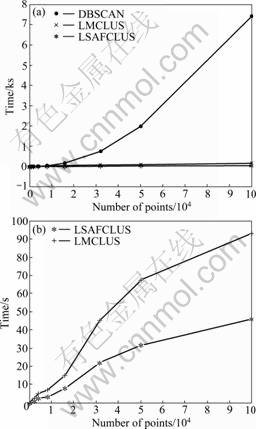
Fig.3 Scalability runtime vs data set size: (a) DBSCAN in comparison with LSAFCLUS and LMCLUS; (b) LSAFCLUS in comparison with LMCLUS

Fig.4 Scalability runtime vs dimensionality of data
Fig.4 shows that the computing complexities of all the three methods are linearly correlated with the dimension of data. LSAFCLUS is the fastest one, followed by LMCLUS; and DBSCAN is the slowest one. In general, the performance of LSAFCLUS is far superior to that of LMCLUS and DBSCAN in terms of runtime. LSAFCLUS is superior over DBCAN in scalability because the runtime of DBSCAN is linearly correlated with the square of the data set size while the runtimes of LSAFCLUS is linear correlated with the data set size. LSAFCLUS is superior over LMCLUS in scalability because LSAFCLUS uses spatial neighbor information to form the original line manifold and adopts the tactic of updating translation vector and eigenvector to find suitable line manifold cluster, while LMCLUS uses the tactic of sampling to find the suitable line manifold cluster. Otherwise, as to the forming of higher dimensional linear manifold cluster, LMCLUS still takes the tactic of sampling which brings large increase of runtime (the rise of the dimension of the linear manifold leads large increase to the sampling times), while LSAFCLUS just simply combines the results of line manifold clusters according to lemma 2 and its extension which spends only very short time. Therefore, LSAFCLUS has good scalability, which is suitable for high dimensional data.
4.3 Real data
Two real datasets are used for our study. The first one is wine recognition data [21]. This data set is about the chemical analysis of Italian wines grown in the same region in Italy but derived from three different cultivars and consists of 13 constituents in each of the three types of wines, which have 59, 71 and 48 instances, respectively. This data set was taken as the first real test data set.
The second data set is a gene expression data set of yeast [22], which measures the expression of genes with 70 measurements for each gene compiled from four time courses during the cell-cycle. This data set has missing values. Before clustering, the missing values were imputed by LSimpute method [23]. 367 genes belonging to five significant function classes are selected from the whole gene set as the second real test data set. The third real test data set consists of the 367 genes that are used in the second data set and another 37 genes as noise that are randomly sampled from the remaining genes. Table 4 presents the cluster accuracy of DBSCAN, LMCLUS and LSAFCLUS in the three real test data sets.
It can be seen from Table 4 that, compared with the other two methods, LSAFCLUS is able to achieve more accurate results in different data sets with different characteristics. These results confirm the suitability of LSAFCLUS previously observed on the synthetic data.
Table 4 Cluster accuracy comparison between LSAFCLUS and other two clustering methods in real test data sets

All the three methods partition the second real test data set into five clusters. DBSCAN and LMCLUS yield moderate accuracy, and LSAFCLUS yields high accuracy, which presents that clustering methods are useful for finding functional gene clusters from gene expression data. As to the third real test data set, DBSCAN and LMCLUS perform poorly, while LSAFCLUS still performs very well. This result demonstrates that when noise gene is added, DBSCAN and LMCLUS are not suitable any more, and LSAFCLUS is suitable for the data with noise. Since gene expression data are of high dimension and a lot of noise, LSAFCLUS is able to handle the clustering tasks for the gene expression data.
5 Conclusions
(1) A new clustering method, LSAFCLUS, which is based on the concept of linear manifolds, is proposed. It clusters a set of points compact around a linear manifold, which are able to capture all kinds of correlations in the data.
(2) LSAFCLUS, as a linear manifold clustering method, only searches the line manifolds rather than high dimensional linear manifolds. By doing so, the searching procedure becomes very fast, which largely decreases the computation time. Otherwise, LSAFCLUS constructs high dimensional manifold clusters by fusing line manifold clusters together under a theoretical foundation, which guarantees the clustering accuracy of LSAFCLUS for data embedded in high dimensional linear manifold.
(3) LSAFCLUS uses both the orthogonal distance and the tangent distance as the linear manifold distance metrics and makes full use of spatial neighbor information during the line manifold searching procedure, which not only enhances the clustering accuracy, but also guarantees the robustness of LSAFCLUS.
(4) The clustering results on real and synthetic data sets demonstrate that LSAFCLUS outperforms LMCLUS and DBSCAN in terms of accuracy and computation time. Otherwise, LSAFCLUS is able to obtain high clustering accuracy for various data sets with varying data set size, manifold dimension and noise ratio, which confirms the suitability of LSAFCLUS on high dimensional data with noise.
References
[1] Agrawal R, Gehrke J, Gunopulos D, RAGHAVAN P. Automatic subspace clustering of high dimensional data [J]. Data Mining and Knowledge Discovery, 2005, 11(1): 5-33.
[2] WITTEN D M, TIBSHIRANI R. A framework for feature selection in clustering [J]. J Am Stat Assoc, 2010, 105(490): 713-726.
[3] ZHENG F, SHEN X, FU Z, ZHENG S, LI G. Feature selection for genomic data sets through feature clustering [J]. Int J Data Min Bioinform, 2010, 4(2): 228-240.
[4] Liu H, Yu L. Toward integrating feature selection algorithms for classification and clustering [J]. IEEE Trans Knowledge and Data Eng, 2005, 17(3): 1-12.
[5] Haque P E, Liu H. Subspace clustering for high dimensional data: A review [J]. ACM SIGKDD Explorations Newsletter, 2004, 6(1): 90-105.
[6] HIRSCH M, SWIFT S, LIU X. Optimal search space for clustering gene expression data via consensus [J]. J Comput Biol, 2007, 14(10): 1327-1341.
[7] Agrawal R, Gehrke J, Gunopulos D, RAGHAVAN P. Automatic subspace clustering of high dimensional data for data mining applications [C]// Proceedings of the ACM SIGMOD International Conference on Management of Data. New York: ACM Press, 1998: 94-105.
[8] Pham D T, Afify A A. Clustering techniques and their applications in engineering [C]// Proceedings of the Institution of Mechanical Engineers. Washington: Professional Engineering Publishing, 2007: 1445-1459.
[9] Kailing K, Kriegel H P, Kroger P. Density-connected subspace clustering for high-dimensional data [C]// Proc Fourth SIAM Int’l Conf Data Mining. German: Lake Buena Vista FL, 2004: 246-257.
[10] Aggarwal C C, Wolf J L, Yu P S, Procopiuc C, PARK J K. Fast algorithms for projected clustering [C]// Proceedings of the 1999 ACM SIGMOD International Conference on Management of Data. New York: ACM Press, 1999: 61-72.
[11] Aggarwal C C, Yu P S. Finding generalized projected clusters in high dimensional spaces [C]// Proceedings of the 2000 ACM SIGMOD International Conference on Management of Data. New York: ACM Press, 2000: 70-81.
[12] Procopiuc C M, Jones M, Agarwal P K, MURALI T M. Monte Carlo algorithm for fast projective clustering [C]// Proceedings ACM SIGMOD. New York: ACM Press, 2002: 418-427.
[13] Lung M, Mamoulis N. Iterative projected clustering by subspace mining [J]. IEEE Trans Knowledge and Data Eng, 2005, 17(2): 176-189.
[14] Cheng Y, Church G M. Biclustering of expression data [C]// Proceedings of the Eighth International Conference on Intelligent Systems for Molecular Biology. La Jolla, California: AAAI Press, 2000: 93-103.
[15] Yang J, Wang W, Wang H, YU P. δ-clusters: Capturing subspace correlation in a large data set [C]// Proceedings of the 18th International Conference on Data Engineering. San Jose, CA: ICDE Press, 2002: 517-528.
[16] Harpaz R, Haralick R. Exploiting the geometry of gene expression patterns for unsupervised learning [C]// Proceedings of the 18th International Conference on Pattern Recognition. Hong Kong: IEEE Computer Society Press, 2006: 670-674.
[17] Haralick R, Harpaz R. Linear manifold clustering in high dimensional spaces by stochastic search [J]. Pattern Recognition, 2007, 40(10): 2672-2684.
[18] DENG Hua, WU Yi-hu, DUAN Ji-an. Adaptive learning with guaranteed stability for discrete-time recurrent neural networks [J]. Journal of Central South University of Technology, 2007, 14(3): 685-690.
[19] ZHOU Xian-cheng, SHEN Qun-tai, LIU Li-mei. New two-dimensional fuzzy C-means clustering algorithm for image segmentation [J]. Journal of Central South University of Technology, 2008, 15(6): 882-887.
[20] Kittler J, Illingworth J. Minimum error thresholding [J]. Pattern Recognition, 1986, 19: 41-47.
[21] AEBERHARD S, COOMANS D, VEL O. The classification performance of RDA [R]. North Queensland: James Cook University of North Queensland, 1992: 92-101.
[22] SHAPIRA M, SEGAL E, BOTSTEIN D. Disruption of yeast forkhead-associated cell cycle transcription by oxidative stress [J]. Mol Biol Cell, 2004, 15(12): 5659-5669.
[23] Trond B, Bjarte D, Inge J. LSimpute: Accurate estimation of missing values in microarray data with least squares methods [J]. Nucleic Acids Research, 2004, 32(3): e34.
(Edited by YANG You-ping)
Foundation item: Project(60835005) supported by the National Nature Science Foundation of China
Received date: 2009-11-26; Accepted date: 2010-03-25
Corresponding author: LI Gang-guo, Doctoral candidate; Tel: +86-731-84574991; E-mail: ligangguo1982@126.com

