J. Cent. South Univ. Technol. (2008) 15(s1): 346-350
DOI: 10.1007/s11771-008-378-z

Feature of resistivity response of slope from steady to unsteady
XIE Zhong-qiu(谢忠球)1, ZHANG Yu-chi(张玉池)2,
WEN Pei-lin(温佩琳)3, DUAN Liang-liang(段靓靓)1
(1. College of Civil Engineering, Architecture and Mechanics,Central South University of Forestry and Technology, Changsha 410004, China;
2. Guilin Institute of Geology for Mineral Resources, Guilin 541004, China;
3. School of Infor-Physics and Geomatics Engineering, Central South University,Changsha 410083, China)
Abstract: Using resistivity as index and referring to the law about effect of slope to resistivity, the apparent resistivities of geophysical model concerned with unsteady rock type slope failure were calculated systematically by using the boundary integral equation method. After studying the feature of resistivity response of slope failure, the variety of resistivity during evolution of slope from steady to unsteady was found and the characteristics of resistivity response about slope failure was concluded. These make electrical exploring method for detecting the slip plane or structural plane of slope failure, evaluating the stability of the slope, and forecasting slope failure become true.
Key words: slope failure; geophysical feature; feature of resistivity response; forecasting of slope failure
1 Introduction
The slope failure will undergo the preparation, production and stabilization, which includes the physical and mechanical courses of slope creep, formation of slide surface, slide under losing stabilization, stabilization after slide etc. During all these courses, the change of physical field is accompanied. Not only the interface position of the slope failure can be detected but also the available theory criterion of forecasting the slope failure can be provided according to the response characteristic of resistivity in the course of slope failure[1-3].
Numerical calculation was carried out by using the method of boundary integral equation. The response characteristic of electric field during the course of the slope failure was researched. The variety of resistivity during evolution of slope from steady to unsteady was found.
2 Research methods
2.1 Numerical calculation models
According to the physics feature for slope failure evolution and the characteristic of engineering geology, the slope can be divided into three layers in this model.
In order to research, hypothesizes are given as follows. 1) Superstratum and understratum medium of the slope body can not be compressed, and the physical property is isotropy and homogeneous. 2) The physical property of the second layer is not evenly changed. For the convenience of calculation, this layer can be divided into three sections, namely, main slippage section, skid resistance section and traction section. The physical property of every section is homogeneous. 3) The thickness of the second layer keeps invariable.
Three-dimensional geology bodies Ω1 and Ω2 with two resistivities ρ1 and ρ2 in homogeneous halfspace Ω with resistivity of ρ are supposed. The boundary integral equation can be deducted as follows[4-8]:

 (1)
(1)

 (2)
(2)
The expression of electric potential U(P) at random point P on the ground is:

 (3)
(3)
where j1 and j2 are potentials produced by the point charge on the ground, S1 and S2; U1 and U2 are electric potential distributions on S1 and S2, respectively;  and
and  are the solid angles expanded by some point on boundary surface for the area; S1 and S2 are the exteriors after P1 and P2 eliminating Ω1 and Ω2, respectively.
For the geology body model with random shape, its surface cannot be expressed by analytical form, therefore, integral equation can only be used for numerical solution method. Dividing S1 and S2 to minor rectangle units, and its corresponding boundary integral equation can be dispersed as:

 (4)
(4)

 (5)
(5)
The expression of electric potential U(P) at random point P on the ground can be dispersed for:

 (6)
(6)
Using the above methods, the values of electric potential at random point on the ground of geology body model with random shape in homogeneous halfspace can be calculated, and the values of apparent resistivity can be obtained.
2.2 Choose of model parameter
According to the analysis of engineering geology characteristic, weak intercalated layer with unfavorable geology for the slope may be clay band, complete weathering rock interlayer, argillization interlayer, crash silt-laden layer and soft rock interlayer in rock slope; clay soft interlayer in soil-rock slope; strip sand gravel aquifer and clay soft interlayer in soil slope. Under the action of water, water enrichment area of weak intercalated layer becomes strain attenuation, along with the change of physical property, viz. resistivity begins to diminish. Along with the increase of water content and degree of saturation, the resistivity of weak intercalated layer such as clay, sand and silt will be reduced related with power function. Approaching to this saturation, current is conducted by pore water, and its resistivity is inclined to stabilize to the resistivity of pore water.
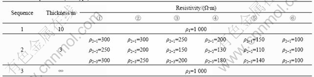
Taking rock model as example for analysis and calculation, the designs of the second layer of matter properties of every geoelectricity models for slope failure are accordant. The second layer of matter properties is divided into three sections: skid resistance section, main slide section and traction section, of which the resistivity ρ2-1 of skid resistance section is changed from 100 Ω?m to 300 Ω?m, ρ2-2 of main slide section is changed from 100 Ω?m to 250 Ω?m, and ρ2-3 of traction section is changed from 100 Ω?m to 300 Ω?m. The thickness is 3.0 m, and the resistivities of superstratum and substratum are homogeneous. Other parameters of the geoelectricity models are designed as follows. The thickness of superstratum is 10 m, the resistivity is 1 000 Ω?m, the thickness of substratum is ∞, and the resistivity is 1 000 Ω?m, as listed in Table 1.
Table 1 Model parameter (rock type)
3 Analysis for resistivity response charac- teristic
Using established physical model, isoline section diagrams of apparent resistivity obtained from numerical calculation are shown in Figs.1-6.
In Fig.1, the resistivities of every section in the second layer are ρ2-1=300 Ω?m, ρ2-2=250 Ω?m and ρ2-3= 300 Ω?m. Because of the infiltration of rainwater and
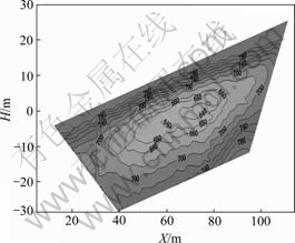
Fig.1 Apparent resistivity isoclines of slope failure model
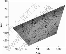
Fig.2 Apparent resistivity isoclines of slope failure model

Fig.3 Apparent resistivity isoclines of slope failure model

Fig.4 Apparent resistivity isoclines of slope failure model
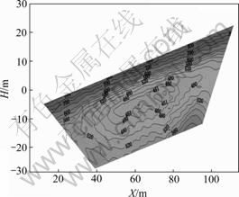
Fig.5 Apparent resistivity isoclines of slope failure model

Fig.6 Apparent resistivity isoclines of slope failure model
surface water, the resistivity ρ2-2 begins to reduce while ρ2-1 and ρ2-3 are constant, indicating the commencement of slope failure (initial state). As shown in Fig.1, low resistance abnormal distribution of apparent resistivity can be seen, in which inclined banded shape appears. The isoclines of apparent resistivity are shown as regular and inclined oval, and the direction is the same as the inclined direction of the second matter properties. The isoclines of the apparent resistivities with 660 Ω?m and 700 Ω?m appear in a oval shape, where position distribution of the major axis projecting on horizontal plane is between 42-85 m and 30-103 m, and the ratio of major axis to minor axis is about 0.23 and 0.26. The abnormal minimum value of apparent resistivity is 637 Ω?m, and the depth of abnormal depth is about 19 m.
In Fig.2, the resistivities of every section in the second layer are ρ2-1=300 Ω?m, ρ2-2=200 Ω?m and ρ2-3= 250 Ω?m. Because of the decrease of the resistivities of the second layer (ρ2-2 and ρ2-3), in the profile of apparent resistivity isoclines, abnormal low resistance with inclined banded shape becomes much obvious, and apparent resistivity oval isoclines become more elongated. The isoclines of apparent resistivities with 600 Ω?m and 660 Ω?m are shown as ellipse, where position distribution of the major axis projecting on horizontal plane is between 48-82 m and 37-110 m, and the ratio of major axis to minor axis is about 0.23 and 0.22. The abnormal minimum value of apparent resistivity is 588 Ω?m, and the depth of abnormal depth is about 19 m.
In Fig.3, the resistivities of every section in the second layer are ρ2-1=250 Ω?m, ρ2-2=150 Ω?m and ρ2-3= 200 Ω?m. The resistivity ρ2-1 begins to decline, which illuminates that the stain generates in skid resistance section and the slope starts to lose stability. Because of the decrease of the resistivities of the second layer (ρ2-2 and ρ2-3), in the profile of apparent resistivity isoclines, abnormal low resistance with inclined and elongated banded shape becomes much obvious. The abnormal minimum value of apparent resistivity falls to 516 Ω?m, and the depth of abnormal depth is about 19 m. The isoclines of apparent resistivities with 540 Ω?m and 600 Ω?m are shown as ellipse, where position distribution of the major axis projecting on horizontal plane is between 40-84 m and 40-110 m, and the ratio of major axis to minor axis is about 0.28 and 0.21.
In Fig.4, the resistivities of every section in the second layer are ρ2-1=200 Ω?m, ρ2-2=130 Ω?m and ρ2-3= 180 Ω?m. Because of the decrease of the resistivities of the second layer, in the profile of apparent resistivity isoclines, abnormal low resistance with inclined banded shape becomes much elongated. The abnormal minimum value of apparent resistivity falls to 486 Ω?m, and the depth of abnormal depth is about 19 m. The isoclines of apparent resistivities with 500 Ω?m and 540 Ω?m are shown as ellipse, where position distribution of the major axis projecting on horizontal plane is between 47-81 m and 41-96 m, and the ratio of major axis to minor axis is about 0.24 and 0.26.
In Fig.5, the resistivities of every section in the second layer are ρ2-1=150 Ω?m, ρ2-2=110 Ω?m and ρ2-3= 140 Ω?m. Because of the decrease of the resistivities of the second layer, in the profile of apparent resistivity isoclines, abnormal low resistance with inclined banded shape becomes much elongated. The abnormal minimum value of apparent resistivity falls to 435 Ω?m, and the depth of abnormal depth is about 19 m. The isoclines of apparent resistivities with 480 Ω?m and 500 Ω?m are shown as ellipse, where position distribution of the major axis projecting on horizontal plane is between 41-95 m and 37-110 m, and the ratio of major axis to minor axis is about 0.21 and 0.22.
In Fig.6, the resistivities of every section in the second layer are ρ2-1=ρ2-2=ρ2-3=100 Ω?m. The resistivities of ρ2-1, ρ2-2 and ρ2-3 fall to 100 Ω・m, which indicates that the slope has already lost stability. In the profile of apparent resistivity isoclines, abnormal low resistance appears in inclined and wafering ellipse, and multiple local abnormity exists. The abnormal minimum value is 396 Ω?m, and the depth of abnormal depth is about 19 m. The isoclines of apparent resistivities with 415 Ω?m are shown as regular long ellipse, and the ratio of major axis to minor axis is about 0.09.
From the result of the analysis, it can be inferred that because of the decrease of the resistivities of the second layer, the abnormal minimum value of the resistivity gradually turns low, the range of abnormal low resistance with inclined banded shape gradually becomes wider, and the ratio of major axis to minor axis becomes lower. According to this feature, the abnormal variety rules of the resistivities during the evolution course of rock slope failure can be obtained. By the action of groundwater, the stain attenuation becomes much enhanced. The resistivities of the weak intercalated layer in the second layer are reduced. The abnormal minimum value of the resistivity gradually turns low. The range of abnormal low resistance with inclined banded shape gradually becomes wider. And the ratio of major axis to minor axis becomes lower. Meanwhile, it shows that the lower the abnormal minimum value of apparent resistivity is, the wider the range of abnormal low resistance with inclined banded shape is, the lower the ratio of major axis to minor axis is, and the easier the rock slope failure takes place.
4 Conclusions
Based on the feature of resistivity response of slope failure, the variety of resistivity during evolution of slope from steady to unsteady was found and the characteristics of resistivity response about slope failure was concluded. These make electrical exploring method for detecting the slip plane or structural plane of slope failure, evaluating the stability of the slope, and forecasting slope failure become true. The profile observation of the resistivity in same profile at different periods and different seasons can provide the criterion of analysis, design and construction of slope failure.
References
[1] ZHANG Yu-chi, WEN Pei-lin. Resistivity responding characteristics reflecting soil slope instability [J]. Mineral Resources and Geology, 2007, 21(5): 573-575. (in Chinese)
[2] ZHANG Yu-chi, WEN Pei-lin, ZHOU Yi, LI Ye-Jun. The application of integrated geophysical techniques to the investigation of landslide geological disasters [J]. Geophysical & Geochemical Exploration, 2007, 31(S): 9-10. (in Chinese)
[3] XIE Zhong-qiu, WEN Pei-lin, DING Ke. Anisotropy characteristics testing for structure plane of slope rock mass and its stability [J]. Journal of Central South University: Science and Technology, 2006, 37(1): 160-163. (in Chinese)
[4] BAO Guang-shu, SUN Zi-ying. Space location of objective bodies under ground using boundary integral equation method [J]. Journal of Central South University of Technology, 2000, 31(2): 102-105. (in Chinese)
[5] RUAN Bai-rao, XIONG Bin. A finite element modeling of three-dimensional resistivity sounding with continuous conductivity [J]. Chinese Journal of Geophysics, 2002, 45(1): 131-138. (in Chinese)
[6] DIETER, PATESON K N R, GRANT F S. IP and resistivity type curves for three-dimension bodies [J]. Geophysics, 1969, 34: 615-632.
[7] TING S M, HOHMANN G W. Integral equation modeling of three-dimensional magnetotelluric response [J]. Geophysics, 1981, 46(2): 182-197.
[8] XIONG Zong-hou. Electromagnetic modeling of 3-D structures by the method of system iteration using integral equations [J]. Geophysics, 1992, 57(12): 1556-1561.
(Edited by YANG Bing)
Foundation item: Project(07JJ6072) supported by the Natural Science Foundation of Hunan Province, China
Received date: 2008-06-25; Accepted date: 2008-08-05
Corresponding author: XIE Zhong-qiu, PhD; Tel: +86-13973179389; E-mail:zqxie8@163.com

