J. Cent. South Univ. (2017) 24: 2028-2034
DOI: https://doi.org/10.1007/s11771-017-3612-8

Model predictive control synthesis algorithm based on polytopic terminal region for Hammerstein-Wiener nonlinear systems
LI Yan(����)1, CHEN Xue-yuan(��ѩԭ)1, MAO Zhi-zhong(ë־��)2
1. AVIC Aerodynamics Research Institute, Aviation Key Laboratory of Science and Technology on
Aerodynamics of High Speed and High Reynolds Number, Shenyang 110034, China;
2. School of Information Science and Engineering, Northeastern University, Shenyang 110004, China
 Central South University Press and Springer-Verlag GmbH Germany 2017
Abstract: An improved model predictive control algorithm is proposed for Hammerstein-Wiener nonlinear systems. The proposed synthesis algorithm contains two parts: offline design the polytopic invariant sets, and online solve the min-max optimization problem. The polytopic invariant set is adopted to replace the traditional ellipsoid invariant set. And the parameter-correlation nonlinear control law is designed to replace the traditional linear control law. Consequently, the terminal region is enlarged and the control effect is improved. Simulation and experiment are used to verify the validity of the wind tunnel flow field control algorithm.
Key words: Hammerstein-Wiener nonlinear systems; model predictive control; polytopic terminal constraint set; parameter- correlation nonlinear control; stability; linear matrix inequalities (LMIs)
1 Introduction
In practical industrial processes, many nonlinear systems can be represented as Hammerstein-Wiener systems [1, 2]. Because two nonlinearities and input/output constraints exist in Hammerstein-Wiener systems, the design of controller is very difficult [3, 4].
In recent years, model predictive control (MPC) has attracted extensive attentions for Hammerstein-Wiener systems [5, 6]. BLOEMEN [7] presented a constrained MPC algorithm. However, online computational load is too large. Assuming that a part of online calculation is converted into the corresponding offline calculation, the online calculation will be reduced. Based on above thought, KOUVARITAKIS et al [8] presented a synthesis MPC algorithm. The approaches contain two parts: offline construct the ellipsoid invariant sets, and online solve the min-max optimization problem. Then the computational burden is reduced. But the terminal set is invariant. In Ref. [9], the terminal set is variable. The control effect is improved. DING and YANG [10] adopted a series of invariant sets to replace the single terminal set. Then, the control performance is better. However, all the above methods [7-10] adopted the ellipsoid sets and the linear feedback control law.
In this work, the improved model predictive control synthesis algorithm is proposed. In the proposed algorithm, the polytopic invariant set is adopted to replace the traditional ellipse invariant set. Moreover, the nonlinear control law is designed to replace the traditional linear control law. Consequently, the terminal region is enlarged and the control effect is improved.
2 Hammerstein-Wiener systems
Hammerstein-Wiener systems are given in Fig. 1.
In Fig, 1, the known input nonlinearity is given as
 (1)
(1)
where 
 f(u) is continuous, monotone and invertible.
Linear time invariant (LTI) subsystem is given as
 (2)
(2)
where 


The known output nonlinearity is as follows:
 (3)
(3)
where  h(w) is continuous, monotone and invertible.
The input and output constraints are written as

Fig. 1 Hammerstein-Wiener nonlinear systems
 (4)
(4)
 (5)
(5)
where


From Eq. (1), the inverse function is given as
 (6)
(6)
In equilibrium neighbourhood, we have [11]:
 (7)
(7)
where  is partial derivative matrix;
 r1=1, 2, ��, m; r2=1, 2, ��, m;


In a similar way, Eq. (3) can be given as
 (8)
(8)
where is partial derivative matrix;
  s1=1, 2, ��, p; s2=1, 2, ��, p;


3 MPC synthesis approach
Assume that the equilibrium point of Hammerstein-Wiener systems are the origin. The original optimal control problem is given as
 (9)
(9)
subject to Eqs. (4), (5), where Ry and Ru are positive definite matrices.
Define the polytopic set as
 (10)
(10)
where V is the coefficient matrix.
Define Lyapunov function as
 (11)
(11)
Then, we impose the following constraint:

 (12)
(12)
where ��>0.
Sum Inequation (12) from i=N to i=��, we have:
 (13)
(13)
From Formulae (9) and (13), we have:

 (14)
(14)
subject to Formulae (4) and (5).
3.1 Off-line construction of a series of polytopic terminal constraint sets
In practice,  and
and  can be identified. Then the nonlinear control law
  is given as
 (15)
(15)
where 


The above parameters satisfy constraints:
 (16)
(16)
 (17)
(17)
 (18)
(18)
From Formulas (7), (8), (15)-(18) and (12), the following formula can be satisfied:


 (19)
(19)
In order to obtain Eq. (10), we need optimize individual vertex successively. For the initial polytope ��0, optimizing vertex  of ��1 can be written as maximizing vol(��1-��0). Denoting Xl,g as the matrix, in which columns formed from gth facet vertices:
  Because Xl,g is independent of , maximizing
  is equivalent to minimizing

Theorem 1: Given the initial upper bound ��(0) and the initial polytopic invariant set 
 with Constraints (4), (5) and (19). Let l=1. Update the vertex
  of ��0 as follows:

 (20)
(20)
subject to

 (21)
(21)
 (22)
(22)
 (23)
(23)
Then the vertex of ��1 and the corresponding control variable  will be obtained. And the polytopic invariant set ��1 is maximum with upper bound ��(0).
Proof: Given the initial upper bound ��(0) of ��1.
From Formula (19), we can see that


(24)
Let  and
and  is contained in
  (24) will satisfy when

(25)
Moreover, the vertex and the corresponding control variable of ��1 satisfy constraints (4) and (5).
As a result, the polytopic set ��1 is the maximized polytopic invariant set with the upper bound ��(0).
Algorithm 1: Maximize polytopic invariant set ��1
Step 1: Given the initial upper bound ��(0) and the initial polytopic invariant set 
 with constraints (4), (5) and (19). Let l=1.
Step 2: Solve Formula (20), then the vertex of ��1 and the corresponding control variable will be obtained.
Step 3: If  , then stop; else, let l=l+1 and return to Step 2.
Remark 1: On the premise of polytopic shape fixation, the vertex in Algorithm 1 can be represented as  where is the vertex of ��0. Then the maximum polytopic invariant set ��1 can be computed by solving


 subject to Formulas (21)- (23). Then the calculation is reduced.
Algorithm 2: Offline construct sequence of polytopic invariant sets
Step 1: Given the initial polytopic invariant set  with the constraints (4), (5) and (19). And given the upper bounds
 . Let
. Let 
Step 2: In Algorithm 1, the upper bound ��(0) is replaced by  , the initial polytopic invariant set
  is replaced by
 . The vertex is replaced by
  The parameters
  are replaced by
 Compute
 using Algorithm 1 or Remark 1, then
  of polytopic invariant set
  is obtained.
Step 3: If  then stop; else, let
  and return to Step 2.
3.2 Online synthesis of min-max optimization problem
From Formulas (2), (7) and (8), we have:


 (26)
(26)

 (27)
(27)


 (28)
(28)
or equivalently
 (29)
(29)
 (30)
(30)
 (31)
(31)
where x(k) is the initial state; 

 and
and  are corresponding to the matrices in Formulas (26)-(28).

Consequently, the system of Formulas (29)-(31) is contained in
 (32)
(32)
Substituting Formula (32) into (14), we have:

 (33)
(33)
From Formula (2), the state prediction values are given as
 (34)
(34)
or equivalently
 (35)
(35)
where 


 and
and  are matrices corresponding to Formula (34).
From Formulas (14) and (35), we have:
 (36)
(36)
From Formulas (10) and (35), the terminal state satisfies:
 (37)
(37)
For 
 , we have:
 (38)
(38)
where  and
and  are compared by
 , respectively.
Substituting (30) into (5), we have:
 (39)
(39)
where  and
and  are compared by
 respectively.
Algorithm 3: Online compute the control laws 
Step 1: For the initial state x(k), the terminal state  can be solved from Formula (35).
Step 2: If system constraints and terminal constraint are satisfied, the control laws  can be solved by
 (40)
(40)
subject to Formulas (33), (38), (39), (41) and (42).
 (41)
(41)
 (42)
(42)
Step 3: Implement  .
.
3.3 Entire MPC optimization problem
Sum up sections 3.1 and 3.2, the steps of the entire synthesis MPC algorithm can be described as follows:
Step 1: For x(k), can be solved from Formula (35).
Step 2: If N>1, the variable horizon MPC is used to solve Formula (40), let N=N-1, then apply  else, if N=1, the fixed horizon MPC is used to solve Formula (40), then apply .
Step 3: Let k=k+1 and repeat Step 2 until the state return to the equilibrium point.
4 Stability analysis
Theorem 2: For Hammerstein-Wiener systems, the improved constrained MPC synthesis approach in Section 3.3 can guarantee closed-loop asymptotic stability, once a feasible solution is found at the initial time.
Proof: For the initial state, the initial optimization problem will be solved with horizon N. The feasible solution at time k is represented as and
and 
 The terminal state satisfies
At next time k+1, the horizon is reduced to N-1, then the feasible solution can be given as  and
and 

When N=1, variable horizon becomes fixed horizon. Assume that N=1 at time k, the feasible solution is and  . The performance index is given as

 (43)
(43)
Then, at next time k+1, we have:
 (44)
(44)
The feasible solution of control law is given as

 (45)
(45)
where


 satisfies:
 (46)
(46)
 (47)
(47)
 (48)
(48)
From Formulas (14) and (44)-(48), we have:


 (49)
(49)
Based on Formula (12), the following holds:


 (50)
(50)
From Formulas (43), (49) and (50), it is given that

 (51)
(51)
From Formula (51), we have:
 (52)
(52)
where  is global objective solution.
Consequently, the closed-loop asymptotic stability of the synthesis approach is guaranteed.
5 Example
The flow field control system can be described as Hammerstein-Wiener nonlinear systems in Fig. 2.
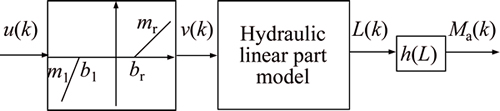
Fig. 2 Mach number control system of wind tunnel
In Fig. 2, the soft inverse function of dead zone can be described as follows [12, 13]:
 (53)
(53)
where  m1=mr=1; br=2; b1=-2.
The discrete hydraulic part is written as [14]
 (54)
(54)
where 


 The sampling period is Ts=0.1 s.
At equilibrium, Mach number is approximated to
 (55)
(55)
where 
The equilibrium point is chosen as: ueq=0; veq=0;  mm/s;
mm/s;  L=200 mm;
  The state transformation is adopted to shift the equilibrium point to the origin. The initial state of the system is given as
  pL=0.5 Pa; L=100 mm. The parameters are Ru=5��10-5, Ry=5��105 and N=3. In actual flow field control, the input constraint is from -10 V to 10 V; the variation range of hydraulic cylinder length is 100 mm to 300 mm and equilibrium point 200 mm; the output constraint is 0.6-1.2. By computing, the polytopic description of the input soft dead zone inverse nonlinearity is
 the polytopic description of the output nonlinearity is

 The number of the polytopic invariant sets is M=1.
In Fig. 3, the terminal sets are compared and the terminal set is enlarged. The reason is stated as follows: the polytopic terminal set is adopted to replace the traditional ellipse terminal set. Then, the terminal constraints are weaker and easier to meet.
Output Mach number is compared in Fig. 4. In Fig. 4, the response speed of proposed algorithm is faster. The reason can be explained that the parameter- correlation nonlinear control law is constructed to replace the traditional linear control law, and then the stability conditions are weaker and easier to meet.
Mach number running curve is given as follows.
From above figure, we can see that in practice experiment, the proposed algorithm is feasible. The flow field control system can run steadily, and the variation range of most Mach number is 0.895-0.905.
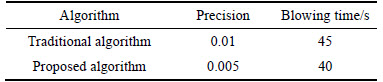
In Table 1, control precision and blowing time are compared. From Table 1, we can see that the control precision is improved and the blowing time is shorten.
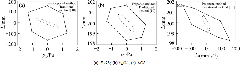
Fig. 3 Comparison of terminal sets on planes:

Fig. 4 Comparison of output Mach number
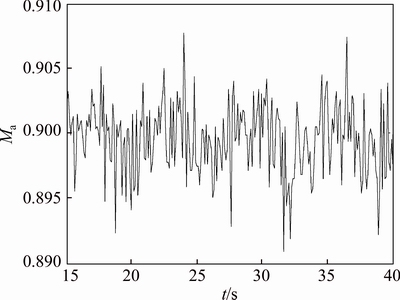
Fig. 5 Running curve of Mach number
Table 1 Comparison of precision and blowing time
6 Conclusions
An improved constrained model predictive control synthesis algorithm is proposed for Hammerstein-Wiener systems. The polytopic invariant set is adopted to replace the traditional ellipse invariant set. Moreover, the nonlinear control law is designed to replace the linear control law. Consequently, the feasible region is enlarged and the control performance is improved.
References
[1] WANG D, DING F. Extended stochastic gradient identification algorithms for Hammerstein-Wiener ARMAX systems [J]. Computers & Mathematics with Applications, 2008, 56(12): 3157-3164.
[2] WANG D, DING F. Hierarchical least squares estimation algorithm for Hammerstein-Wiener systems [J]. IEEE Signal Processing Letters, 2012, 19(12): 825-827.
[3] SUNG S W, JE C H, LEE J, LEE D H. Improved system identificat ion method for Hammerstein-Wiener processes [J]. Korean Journal of Chemical Engineering, 2008, 25(4): 631-636.
[4] PATCHARAPRAKITI N, KIRTIKARA K, MONYAKUL V, CHENVIDHY A D, THONGPRON J, SANGSWANG A. Modeling of single phase inverter of photovoltaic system using Hammerstein-Wiener nonlinear system identification [J]. Current Applied Physics, 2010, 10(3): 532-536.
[5] XI Yu-geng, LI De-wei. Fundamental philosophy and status of qualitative synthesis of model predictive control [J]. Acta Automatica Sinica, 2008, 34(10): 1225-1234.
[6] PATIKIRIKORALA T, WANG L, COLMAN A, HAN J. Hammerstein-Wiener nonlinear model based predictive control for relative QoS performance and resource management of software systems [J]. Control Engineering Practice, 2012, 20(1): 49-61.
[7] BLOEMEN H H J, van den BOOM T J J, VERBRUGGEN H B. Model-based predictive control for Hammerstein-Wiener systems [J]. International Journal of Control, 2001, 74(5): 482-495.
[8] KOUVARITAKIS B, ROSSITER J A, SCHUURMANS J. Efficient robust predictive control [J]. IEEE Transactions on Automatic Control, 2000, 45(8): 1545-1549.
[9] WAN Z, KOTHARE M V. An efficient off-line formulation of robust model predictive control using linear matrix inequalities [J]. Automatica, 2003, 39(5): 837-846.
[10] DING Bao-cang, YANG Peng. Synthesizing off-line robust model predictive controller based on nominal performance cost [J]. Acta Automatica Sinica, 2006, 32(2): 304-310.
[11] LI Yan, CHEN Xue-yuan, MAO Zhi-zhong, YUAN Ping. An improved constrained model predictive control approach for Hammerstein-Wiener nonlinear systems [J]. Journal of Central South University, 2014, 21(3): 926-932.
[12] YAU H T. Generalized projective chaos synchronization of gyroscope systems subjected to deadzone nonlinear inputs [J]. Physics Letters A, 2008, 372(14): 2380-2385.
[13] WANG D, CHU Y, YANG G, DING F. Auxiliary model based recursive generalized least squares parameter estimation for Hammerstein OEAR systems [J]. Mathematical and Computer Modelling, 2010, 52(1): 309-317.
[14] ZHANG You-wang, GUI Wei-hua. Compensation for secondary uncertainty in electro-hydraulic servo system by gain adaptive sliding mode variable structure control [J]. Journal of Central South University of Technology, 2008, 15(2): 256-263.
(Edited by YANG Hua)
Cite this article as: LI Yan, CHEN Xue-yuan, MAO Zhi-zhong. Model predictive control synthesis algorithm based on polytopic terminal region for Hammerstein-Wiener nonlinear systems [J]. Journal of Central South University, 2017, 24(9): 2028�C2034. DOI:https://doi.org/10.1007/s11771-017-3612-8.
Foundation item: Project(61074074) supported by the National Natural Science Foundation, China; Project(KT2012C01J0401) supported by the Group Innovation Fund, China
Received date: 2016-02-22; Accepted date: 2016-05-23
Corresponding author: LI Yan, Senior Engineer, PhD; Tel: +86-24-86566875; E-mail: neu_liyan@163.com

