

J. Cent. South Univ. (2018) 25: 3004-3020
DOI: https://doi.org/10.1007/s11771-018-3970-x

Dynamic friction modelling and parameter identification for electromagnetic valve actuator
SHAO Da(�۴�)1, 2, XU Si-chuan(��˼��)1, 2, DU Ai-min(�Ű���)1
1. School of Automotive Studies, Tongji University, Shanghai 201804, China;
2. Clean Energy Automotive Engineering Center, Tongji University, Shanghai 201804, China
 Central South University Press and Springer-Verlag GmbH Germany, part of Springer Nature 2018
Abstract:
A new modified LuGre friction model is presented for electromagnetic valve actuator system. The modification to the traditional LuGre friction model is made by adding an acceleration-dependent part and a nonlinear continuous switch function. The proposed new friction model solves the implementation problems with the traditional LuGre model at high speeds. An improved artificial fish swarm algorithm (IAFSA) method which combines the chaotic search and Gauss mutation operator into traditional artificial fish swarm algorithm is used to identify the parameters in the proposed modified LuGre friction model. The steady state response experiments and dynamic friction experiments are implemented to validate the effectiveness of IAFSA algorithm. The comparisons between the measured dynamic friction forces and the ones simulated with the established mathematic friction model at different frequencies and magnitudes demonstrate that the proposed modified LuGre friction model can give accurate simulation about the dynamic friction characteristics existing in the electromagnetic valve actuator system. The presented modelling and parameter identification methods are applicable for many other high-speed mechanical systems with friction.
Key words:
Cite this article as:
SHAO Da, XU Si-chuan, DU Ai-min. Dynamic friction modelling and parameter identification for electromagnetic valve actuator [J]. Journal of Central South University, 2018, 25(12): 3004�C3020.
DOI:https://dx.doi.org/https://doi.org/10.1007/s11771-018-3970-x1 Introduction
Friction is always present in all mechanical systems undergoing relative motion in contact. Valvetrain friction is responsible for 18% of the total engine friction loss, varying with design and operating conditions [1]. Camless technologies which often refer to an electromagnetic actuator can not only decrease the friction loss, but also realize fully variable valve parameters (timing, lift and valve duration) to depress the pumping loss and accomplish new thermodynamic and combustion cycle improving the engine efficiency. Friction loss of electromagnetic camless engine may be significantly reduced by removing the moving parts between cam/follower, camshaft bearings, follow/ guide which make a significant contribution to the valvetrain friction. The only contact interface undergoing relative motion exists between valve/ guide interface. This friction affects the performance of the control system, arising positioning errors during the execution of reference trajectory task and deteriorating the stability of the system. In order to improve the performance of the control system, it is necessary to predict the behaviors of friction and compensate it in control algorithm [2, 3].Tremendous efforts have been made to establish an accurate mathematical model of friction behaviors observed in mechanical systems since Coulomb��s hypothesis. These models can be divided into two types: static and dynamic models. Static models can describe the nonlinear behavior between friction force and velocity at a steady state and represent the essential properties of macroscopic friction, such as coulomb friction, viscous friction, static friction and Stribeck effect, but cannot completely describe the complex memory phenomenon about the microscopic presliding regime (hysteretic effect during the switch between stick and slip phases) and macroscopic pure sliding regime (frictional lag, non-reversible friction characteristic). Dynamic models, such as Dahl model, Bliman-Sorine model, LuGre model, GMS model, were developed to capture the above characteristics of the two regimes and their transitions. Among them, the LuGre model proposed by WIT et al [4] can describe the major behaviors observed in experiments, including hysteresis effects during stick-slip transition, presliding displacement, varying break- away force and Stribeck effect, thus has been widely used in control with friction compensation [5�C7]. Nevertheless, there are some intrinsic implementation problems for some applications with a large range of motion speeds, such as electromagnetic valve actuator system presented in this work. It has been reported by FREIDOVICH et al [8] that the discrete observer of internal state may become oscillatory and unstable at high-speed motions. It is suggested to stop integrating the internal state and use its steady-state value for high-speed applications [8]. However, this modification may result in discontinuance of internal state when the velocity transits between low and high ranges according to the opinion of LU et al [9]. In addition, The LuGre model cannot predict accurately the non- reversible hysteresis dynamic friction behaviors in sliding regime at high speeds [10, 11]. STEFA SKI et al [12] confirmed the existence of this non-reversible friction characteristics and proposed that friction depends not only on its velocity but also on its current acceleration in sliding regime. And then, a friction model which had the appearance of an acceleration variable to simulate the non-reversible friction characteristics was proposed [12]. GUO et al [10] proposed a new non-reversible sliding friction model which consists of velocity-dependent part and acceleration-dependent part and had a good fit with experimental data in both sliding and presliding regimes. TRAN et al [13, 14] incorporated a hysteresis function and fluid film friction dynamics into the LuGre model to simulate the observed friction behaviors with a good accuracy in both pre-sliding and sliding regimes of the pneumatic cylinders. SAHA et al [11] modified the LuGre model to capture both clockwise and counter clockwise hysteretic loops in the sliding regime. LI et al [15] modified the LuGre model by taking the external load into consideration to investigate the friction characteristics for giant forging press.
Motivated from these achievements, this work proposes a new friction model based on LuGre model to accurately describe and predict the behaviors of friction in electromagnetic valve actuator system. New model preserves the LuGre��s capacity of simulating the major behaviors observed at low speeds and adds an acceleration- dependent part to capture the velocity hysteresis effect at high speeds. A nonlinear continuous function is employed to make the transition continuous and stop integrating the internal state at high speeds so as to stabilize its observer for real- time implementation.
It is necessary to identify the parameters of the friction model after the model structure is established. Classical identification methods such as least-squares algorithm do not apply directly to the determination of the friction model since friction is a nonlinear phenomenon. Therefore, a special approach to identify the parameters is necessary. The static parameters can be identified from the steady state response experiments by measuring the current and velocity which is kept constant by velocity control loop. However, tremendous quantity of experiments and enormous effort should be made because the experiment for each bi-directional velocity should be done many times to capture the general characteristics of steady-state friction [16]. In addition, the steady state response experiments cannot estimate the dynamic parameters of friction model because there exists an unknown and immeasurable internal state.
Numerous intelligent algorithms, such as particle swarm optimization [17�C19], fruit fly optimization algorithm [20], genetic algorithm [21], artificial bee colony algorithm [22], are used in parameter identification at present. The parameter identification is transformed to the optimal selection by minimizing the objective function. PSO algorithm is a multi-agent parallel, stochastic global search technique that emulates the social behavior of animals such as fish schooling and bird flocking. Compared with the optimization methods mentioned above, PSO algorithm has the ability to converge toward the global solution rapidly and does not require the derivative of the objective function which is difficultly obtained for highly nonlinear systems, thus has received much praise and attention in recent years. However, they are frequently trapped into a local optimum and may cause premature convergence [23].
In this work, an improved artificial fish swarm algorithm (IAFSA) is proposed to identify the parameters of the proposed modified LuGre friction model. Owing to combining with chaotic search and Gauss mutation operator, the IAFSA can increase the diversity of population and probability of jumping out of the local optimum, and thus prompts the population to converge toward the global optimum rapidly. The steady state response experiments are also conducted to obtain the static parameters of proposed modified LuGre friction model. The experimental results are compared with the results from IAFSA to evaluate its effectiveness and accuracy.
As mentioned above, the contributions of this work include: 1) modifying the traditional LuGre friction model to enhance the ability for simulating the velocity hysteresis and stabilizing its discrete observer at high speeds, extending its applicable speed range to high-speed applications, 2) adding the chaotic search and Gauss mutation operator into traditional artificial fish swarm algorithm to improve the capacity for leaping out local optimum and accelerate the convergence velocity toward the global optimum. The remainder of this work is organized as follows: Section 2 describes the electromagnetic valve actuator, the experimental rig and results. In Section 3, the proposed modification to the LuGre friction model is presented based on the experimental results. A new parameter identification algorithm for the modified friction model is given in Section 4. The experimental data and simulation results are presented and discussed in Section 5. Finally, the main conclusions are drawn in Section 6.
2 Test setup and experiments
2.1 Experimental setup
Figure 1 shows a present friction experimental platform including two valve actuators, a single cylinder head, two Mercury 1500S encoder systems for measuring the position of the valves, a 150V DC power, a motion controller board (SPiiPlusEC, ACS), a driver module (UDMmc, ACS) which contains current sensors for measuring the current of voice coil motors (VCM) and a control software SPiiPlus MMI Application Studio. Figure 2 shows the structure of the voice coil electromagnetic valve (VEMA). The VEMA consists of several moving coil windings, a coil carrier, a valve, a spring, several cylindrical permanent magnets, an outer cylindrical shell, an upper coaxial connector, a lower coaxial connector and a glass scale. Several radially-magnetized and axially-magnetized cylindrical permanent magnets constitute the Halbach magnet array to improve the operating- efficiency for maximizing the actuating force. The moving coil assembly is disposed within the annular air gap between the shell and the permanent magnets. The current produces an axial force upon coil abiding by Lorentz Force Principle that actuates the coil and the valve to move along the guide. The axial force can be bi-directional as the direction of the current changes. The magnitude of the axial force is nearly proportional to the magnitude of the current to the VCM. A single spring with low stiffness is used to hold the valve closed when the power is off. Experimental data,e.g., position and current, are sampled at the interval of 0.05 ms (20 kHz). Zero-phase Butterworth low-pass filter is used to reduce the measurement noise of velocity and current.

Figure 1 Schematic diagram of experimental platform
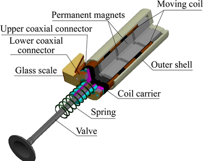
Figure 2 Structure of voice coil electromagnetic valve
In this work, the voice coil motor is used as electromagnetic valve actuator to match the engine��s operating condition. The linear reciprocating motion of electromagnetic valve actuator is characterized by high frequency and high velocity. The motion of the electromagnetic valve actuator can be described by the following equation:
 (1)
(1)
where m is the moving mass combining the valve, the coil and a third of the spring mass; v is the calculated velocity of the valve; S is the measured position of the valve; i is the current through the coil; k is the spring stiffness; const is the pre-deformation of the spring and is set as 6 mm; Ff is the friction between the valve and the guide; fmag(S,i) denotes the force sensitivity function which varys with the current and position. The velocity v and acceleration of the valve are calculated successively by an approximate differentiation of the measured valve position.
To establish the accurate relationship between the current and the axial force, magnetic field simulation and bench test are performed. Magnetic field simulation is applied to analyzing the performance of VEMA utilizing a finite element analysis software (Ansoft��s Maxwell). Figure 3 shows the assembled actuator in a benchtop test for measuring the force curve against position and current. The simulation and experimental results of force curve against position and current are shown in Figure 4 which are in good agreement within an acceptable error. After the establishment of the function fmag(S,i), the electromagnetic force acting on the valve is calculated by measuring the current and position of the VCM. The friction force between the valve and the guide can be calculated by Eq.(1).
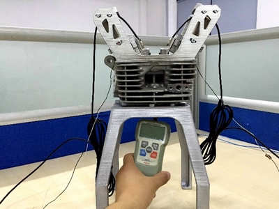
Figure 3 Assembled actuator in benchtop test for measuring force curve against position and current
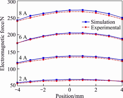
Figure 4 Comparison between simulation and experimental electromagnetic force against position and current
2.2 Experimental results
The valve is controlled to make a sinusoidal movement at different frequencies (1, 5, 10 and 20 Hz) and different magnitudes (2, 4, 6 and 8 mm). The results of the experiment at 1 Hz and 8 mm magnitude for four sinusoidal motion cycles, representing an example of dynamic friction characteristics between velocity and displacement, are presented in Figure 5. Figure 5(a) shows the raw and filtered sinusoidal velocity curve of the valve. Figure 5(b) shows the raw and filtered current curve. Figure 5(c) shows the dynamic friction force�C displacement curve. Figure 5(d) shows the dynamic friction force�Cvelocity curve. Experimental friction behavior from Figure 5(d) reveals a feature mainly combining coulomb and viscous friction effect and it is shown that the dynamic friction force during the acceleration phase is larger than the force during the deceleration phase. The arrows clearly show the dynamic friction force path during the acceleration and deceleration phases. The friction force-velocity curve follows the different paths during the acceleration and deceleration phases forming the clockwise vertical hysteretic loop. The counter- clockwise horizontal hysteresis loop caused by contact compliance during the presliding regime is also clearly visible.
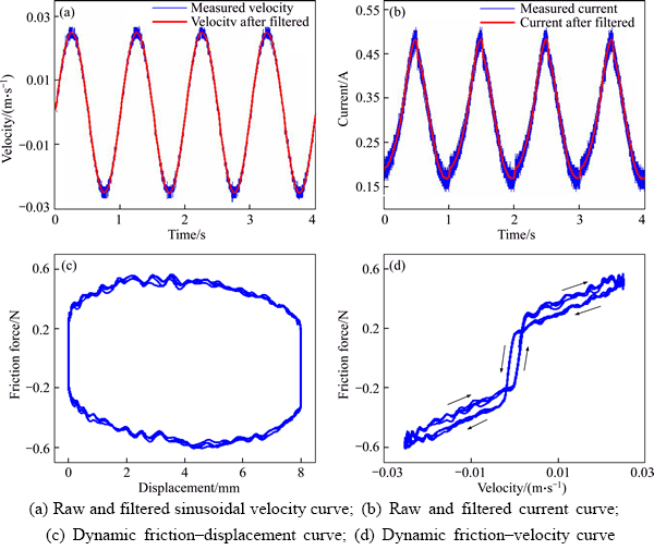
Figure 5 Typical dynamic friction characteristics at 1 Hz and 8 mm magnitude:
Figure 6 presents the measured dynamic friction force-velocity curves at different frequencies (1, 5, 10 and 20 Hz) with a constant magnitude of 8 mm and Figure 7 presents curves with magnitudes of 2, 4, 6, 8 mm at 5 Hz for one sinusoidal motion cycle. It is noticeable that the double hysteretic effect combining with viscous and coulomb friction effect is the main characteristic of dynamic friction existing in electromagnetic valve actuator. The size of the vertical hysteretic loop is increased with the increasing frequency and magnitude. Strictly speaking, it is the acceleration and velocity that are directly responsible for the vertical hysteresis shape. The size of the horizontal hysteresis is almost not changed at the same frequency but different magnitudes and becomes inconspicuous relatively with increasing frequency. The maximum static friction is close to the coulomb friction thus the inconspicuous Stribeck effect is observed.

Figure 6 Measured dynamic friction force�Cvelocity curves at different frequencies (1, 5, 10 and 20 Hz) with a constant magnitude of 8 mm
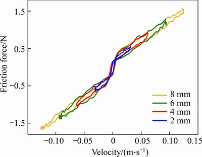
Figure 7 Measured dynamic friction force�Cvelocity curves with magnitudes of 2, 4, 6, 8 mm at 5 Hz
3 Proposed friction model
In this section, the traditional LuGre friction model is presented and the intrinsic implementation problems at high speeds are discussed. A modified LuGre friction model for electromagnetic valve actuator system is then proposed.
The LuGre model proposed by WIT et al [4] can be expressed by the following formulas:
 (2)
(2)
 (3)
(3)
where v is the velocity of linear voice coil motor; z represents the immeasurable internal friction state which can be interpreted as the average bristle deflection; ��0 is the stiffness of the elastic bristles; ��1 is the microdamping of the elastic bristles; ��2 is the viscous friction coefficient; g(v) is a nonlinear function describing a characteristic of the Coulomb friction and the Stribeck effect. Its value lies in the range [Fc, Fs]. A reasonable choice of g(v)is given by
 (4)
(4)
where Fs corresponds to the static friction force; Fcis the Coulomb friction force; vs is the Stribeck velocity coefficient which determines how quickly g(v) approaches Fc; �� is the appropriate fitting parameter. For constant velocity, the steady-state friction force is given by
 (5)
(5)
where sgn( ) is the Signum function, defined by
 (6)
(6)
Based on the experimental data presented in Section 2, the maximum velocity can reach to 0.5 m/s. It is possible to have some implementation problems of LuGre model if the velocity is too large. Firstly, it is shown that the LuGre model is dissipative if ��1(v)<4g(v)/|v|, indicating that the velocity should not exceed a certain value [24]. Moreover, due to the friction state z is immeasurable, it is necessary to construct discretized observer under a certain finite sampling rate to estimate z for dynamic friction compensation. If the velocity is greater than a critical value which is inversely proportional to the stiffness ��0 and sampled time interval, the discrete observer of z will oscillate and grow in magnitude, resulting in the friction model unstable. It is suggested to stop the integration of z and to use its steady-state value zss=Fcsgn(v)/��0 [25], but this may result in discontinuous of internal state z when the speed transits between low and high ranges. Finally, the LuGre model cannot describe the vertical velocity hysteresis during the high speeds due to stopping the integration of state z. Another reason contributing to this phenomenon is that the LuGre model does not include the acceleration variable which is confirmed having impact on the hysteretic memory effect. Taking these into consideration, a modified LuGre model which applies to the application for electromagnetic valve actuator system is established to solve the problems mentioned above. The proposed friction model is given as follows:
 (7)
(7)
 (8)
(8)
 (9)
(9)
 (10)
(10)
 (11)
(11)
where Fd is an acceleration-dependent part containing the velocity and acceleration which are major contributors to vertical hysteresis during the high speed range; ��, ��, vc, as, fa, �� are the fitting parameters of acceleration-dependent part to be identified; a is the current acceleration of the valve;��(v) is a nonlinear continuous switch function with the following properties: ��(v)��1 if |v|<>1 and ��(v)��0 if |v|>v2, v2>v1>0. Equation (7) will be equivalent to the form of Eq. (2) of the traditional LuGre model at low speeds and turn to zero at high speeds. Thus, the modified LuGre model preserves the LuGre��s capacity of simulating the horizontal hysteresis observed at low speeds and meanwhile can stop integrating the internal state continuously to stabilize its observer when the speed is high enough. Moreover, it just stops updating the internal state z but does not force z to be its static value. Therefore, the observer of z is continuous when the speed transits between low and high ranges. An acceleration-dependent part Fd is added to capture the vertical velocity hysteresis effect during the sliding regime. Thus, due to the existence of ��(v) and Fd, the proposed modified LuGre model solves the implementation problems for traditional LuGre model at high speeds and extends its applicable speed range. For any constant speed motion, the steady-state friction can be obtained by letting a=0 and  The proposed modified LuGre model will transform into exactly the same as the form of Eq.(5).
4 Parameter identification
The parameters of the new proposed model are divided into two groups: the static parameters (Fc, Fs, ��, vs, ��2) and the dynamic parameters (��0, ��1, vc, ��, ��, fa, as, ��). In fact, the friction obtained by experiment described in Section 2 represents an asymmetric phenomenon. Asymmetry is a common property of friction and has been observed experimentally in Ref. [11]. Two different sets of parameter values corresponding to the positive and negative motion directions can be employed respectively to describe the asymmetry. That is to say, there are nine static parameters 
 and eleven dynamic parameters (��0, ��1,
 ��, ��, ��) constituting a 20-dimension space to be identified. The computation load for the identification is very large. The usual solution is to divide the identification procedure into two steps: firstly, estimate the static parameters based on the steady friction-velocity curve obtained from the steady state response experiments; secondly, identify the dynamic parameters based on the dynamic friction force-velocity curves using the identified parameters in the first step. However, to do this, tremendous quantity of experiments should be performed because the experiment should be done many times at least in each direction of motion to capture the general characteristics of steady-state friction. Moreover, there exists a coupling effect between the static and dynamic parameters causing the identification more complicated. In this section, an artificial fish swarm algorithm, coupled with chaotic search and Gauss mutation operator, is proposed to identify the static and dynamic parameters simultaneously.
Now, suppose the expected parameter vector to be identified is

 (12)
(12)
During the identification process, �� is split into two sections:

 (13)
(13)

 (14)
(14)
Define the state variable vector as
 (15)
(15)
Define the identification error as
 (16)
(16)
where Ff(x) is the dynamic friction force calculated from experimental data;  is the estimated value of Ff(x) substituting �� into the proposed model Eqs. (7) to (11).
The objective function, also called the fitness or food concentration, representing the quality of each AF, is taken as the form as follows:
 (17)
(17)
where N is the number of the data points; i represents the index of the data points. Equation (17) is also known as root mean square error (RMSE). The smaller Y indicates a better matching between the simulation results and experimental data. The optimization target is to minimize the objective function Y.
4.1 Standard artificial fish swarm algorithm
Artificial fish swarm algorithm (AFSA), first proposed by LI [26], is a new self-organized swarm intelligent optimization algorithm imitating the natural fish social behaviors to reach the global optimum.
Suppose that there are n fishes existing in a D-dimensional searching space. The current position of a fish is represented by a vector  where i=(1, 2, ��, n), t represents the current iteration number and
  (l=1, 2, ��, D) is the variable to be optimized.
  represents its current food concentration, where
 is the objective function of the optimization problem. The Euclidean distance between the ith and jth AF is denoted as
 Rand(0, 1) represents a random variable between 0 and 1. Step and Visual are the maximum movement distance and greatest perception distance of an AF, respectively. �� is the crowd factor and �� is the threshold for crowd factor. Some basic fish swarm behaviors used for searching the food are briefly depicted as follows:
1) Preying behavior
Suppose that the current position of an AF is It selects a position
 randomly within the visual distance andis formulated as Eq. (18). If
  in the minimum problem, the AF moves a step from
  to which is formulated as Eq. (19). Otherwise, it selects another state
  randomly and estimates its food concentration. If it does not satisfy after try_number times, it executes random moving behavior which is described in (Step 4).
 (18)
(18)
 (19)
(19)
2) Swarming behavior
Suppose that the current position of an AF is 
 is the number of its neighbors within the Visual distance and
  is the position of its neighbors,
 If
If let
let  If
If in the minimum problem and ��<��, the AF moves a step from to
  which is formulated as Eq. (20). If
  then it executes the preying behavior.
 (20)
(20)
3) Following behavior
Letbe the current position of an AF and suppose is the position of the AF within the Visual distance which has the least
  for the minimum problem and
 is the number of fishes existing within the distance between and
 . If
. If  the AF moves a step from to which can be formulated as Eq. (21). If
  then it executes the preying behavior.
 (21)
(21)
4) Moving behavior
Let be the current position of an AF. It chooses a random position within the Visual distance and moves a step toward this position despite how much the food concentration of that position. This behavior can be formulated as Eq. (22).
 (22)
(22)
5) Bulletin
Bulletin supplies the global information during iterations that guides the social behaviors of fish swarm. The most optimal value of AF swarm during each iteration is recorded in bulletin.
4.2 Proposed improved fish swarm algorithm
Comparing with the traditional bird PSO, the AFSA increases the randomness and uncertainty to improve the ability of jumping out of the local optimum due to the existence of Step and Visual. However, with the dimension of parameter vector increased, there likely are more local optimums. The swarming behavior and following behavior will accelerate converging toward these local optimums causing a slow evolution speed in the late iterations. In order to overcome the deficiency of the standard AFSA, Gauss mutation operator is added in this work to improve the diversity of the AFs when the value of bulletin board changes a little during a certain iteration, and then chaotic search is executed to help AFs to find the global optimum when the value of bulletin board has no change during a certain iteration.
If the value in bulletin board changes a little or its difference is smaller than a given value �� during the 10 iterations, choose ten of the worst AFs to execute Gauss mutation to improve the diversity of population and drive them to unexplored regions of the search space so as to increase the probability to reach the global optimum. To protect the evolutionary process of the AFs after Gauss mutation, it is forbidden for them to mutate again during the 20 subsequent iterations. Gauss mutation is referring to add a random value which is under Gauss probability distribution to each current element of AF��s state vector to create a new offspring. Gauss mutation can be formulated as Eq. (23).
 (23)
(23)
whereis the current position of the AF; N(0, 1) denotes a random number extracted from a Gaussian distribution with mean 0 and standard deviation 1; is the new position after Gauss mutation.
If the value in bulletin board is not changed after the 10 iterations, it manifests that the fish swarm has fallen into a local minimum. Even if the Gauss mutation has been executed on the worst ten AFs to make them get out local optimum easily, then it still has a probability and needs much more iterations to find a new state better than the state of bulletin. The performance of chaotic search is better than random search due to its special characteristics, i.e. ergodicity, pseudo-randomness and irregularity. Coupling these characteristics of chaotic search into the AFSA can help artificial fish swarm to find a new better state than the local minimum promptly and guide the evolution of the whole population. The process of chaotic search is as follows:
1) The current position of the best AF,  , should be mapped to the chaotic variables,
 The mapping can be formulated as Eq. (24):
 (24)
(24)
where al, bl are the minimum and maximum of the lth dimensional variable respectively; c is the iteration index for chaotic search initialized from 0;
  is the lth dimensional chaotic variable,
  .
.
2) The chaotic sequence 
 is produced by Logistic mapping function which is formulated as Eq. (25):
 (25)
(25)
where �� is the control parameter, 0�ܦ̡�4. The chaotic sequence  will be in fully chaotic state when ��=4here. The chaotic behavior is sensitive to the initial value of

 . The irregularly trace of chaotic variable sequence will travel ergodically over the whole space of definition domain.
3) The chaotic sequence should be mapped to the feasible solution space. Here, we restrict the chaotic search to the range between the [�CVisual,Visual] by the following equation:
 (26)
(26)
Calculate the objective function of  and compare with
  Ifis superior to
  update
 and jump out of the chaotic search iteration. Otherwise, do not update
 and turn to Step 2) starting the next chaotic search iteration. If c exceeds the maximum chaotic iteration number, let
  and break out of the chaotic search.
To execute the IAFSA algorithm described above, the implementary procedures of IAFSA algorithm are given as follows:
Step 1: Initializing IAFSA and bulletin board
The parameters listed in Eq. (12) are identified utilizing IAFSA. Each AF represents a different parameter vector ��i which contains 20 parameters to be identified (i=1, 2, ��, n). Initialize each component element of parameter vector ��i with random value between different ranges, 


 The bulletin board is initialized with zero.The total number of AFs is 50; moving step is 0.5; try_number is 3; crowd factor threshold �� is 0.7; �� is 5��10�C6. The maximum iteration number is 1000 and the maximum chaotic iteration number is set to 3000. It is worth mentioning that Visual is a vector rather than a constant value. Each component element of the Visual vector corresponds to the perception space of each dimensional variable

 Vl (l=1, 2, ��, D)=0.6*(bl�Cal).
Step 2: Behavior selection and execution
Calculate the objective function value of every AF and the best value of them is recorded in bulletin board. Every AF executes swarming behavior, following behavior and preying behavior respectively if these behaviors�� conditions are satisfied. Then compare and choose the best result of the three behaviors. If the best result is better than its current state, the AF implements the best behavior.
Step 3: Gauss mutation
If the value in bulletin board changes a little or its difference is smaller than a given value �� during 10 iterations, choose ten of the worst AFs to execute Gauss mutation to improve the diversity of population. Else, go to Step 2.
Step 4: Chaotic search
If the value in bulletin board is not changed after the 10 iterations and the current chaotic iteration number is less than the maximum chaotic iteration number, the best AF implements the chaotic search to find a new better state and updates the bulletin board. Else, turn to step 2.
Step 5: Update bulletin board
Calculate and compare the objective function value of every AF and the best value is updated in bulletin board.
Step 6: Termination condition
The IAFSA algorithm will be stopped if it reaches the predefined maximum iteration number or the value in bulletin board is close to the expected objective function value within an acceptable error. Else, turn to Step 2.
5 Results and discussions
In this section, we first illustrate the performance of the proposed IAFSA algorithm by comparing with the standard AFSA algorithm. The effectiveness of the proposed IAFSA algorithm is validated based on the experimental data from steady state response experiments and dynamic friction experiments. A number of dynamic friction experiments with different sinusoidal excitation displacement magnitudes and different frequencies are implemented to obtain the experimental dynamic friction force�Cvelocity curves. The simulation curves are generated from the proposed modified LuGre friction model using the parameters identified from IAFSA algorithm.
Figure 8 presents the evolutionary process of the objection function value (RSME) versus the iteration number for standard AFSA and proposed IAFSA algorithm at 5 Hz and 8 mm magnitude. Obviously, the convergence speed of IAFSA is faster than AFSA and IAFSA produces a more precision solution than AFSA ultimately. However, in fact, it consumes more computational time than AFSA because the chaotic search and Gauss mutation will demand a certain computational time during an iterative step. Although AFSA demands less computational time, AFSA is easier to be trapped into a local minimum and is almost impossible to get out even if more time resource is given. As shown in Figure 7, the convergence of the AFSA almost stalls after the 580 generations, indicating that it has been trapped into a local minimum. But IAFSA still continues to converge during the almost whole iteration process and the stalling situation lasts no more than 10 iterations before the last 70 iterations, indicating the chaotic search takes effect when the objection function stalls 10 iterations. Chaotic search propels AFs to get out of the local optimum and guides the evolution direction for the whole population forming the continuous optimization process as presented in Figure 7. During the last 70 iterations, the objection function stalls, indicating that a better solution cannot be found by chaotic search within the maximum chaotic iteration number and defined chaotic solution space. It is reasonable to assume that the artificial fish swarm has found the global optimum under the existing constraints. Obviously, if the quality of global optimum obtained from IAFSA is not satisfied, it is suggested to expand the feasible solution space, raise the maximum chaotic iteration number and extend the iteration process. The comparison manifests that the IAFSA has a faster convergence speed, a better optimization precision and improved capacity for leaping out local optimum and finding global optimum. Table 1 presents the values of the identified parameters for modified LuGre model obtained from the IAFSA algorithm.
To verify the performance and accuracy of IAFSA, the steady state response experiments are first implemented to obtain the steady force�C velocity curve. The static parameters extracted from the experimental data are compared with the identified results to evaluate the effectiveness and accuracy of IAFSA algorithm.

Figure 8 Comparison of RMSE versus iteration number based on AFSA and IAFSA algorithm at 5 Hz and 8 mm magnitude
Table 1 Identified parameters for modified LuGre model obtained from IAFSA algorithm

In this experiment, the velocity of the electromagnetic valve was kept constant by velocity control loop. The friction force at that velocity was calculated by measuring the current and displacement of the VCM. By repeating this experiment at 48 bi-directional different velocities in the range from �C0.02 to 0.02 m/s, the steady force�Cvelocity curve is plotted, as shown in Figure 9.

Figure 9 Experimental data and fitted curve for steady force versus velocity
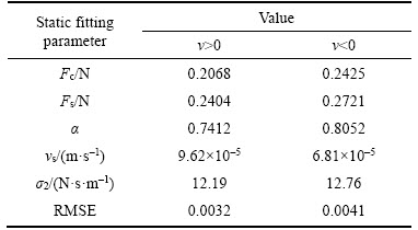
Figure 9 presents the experimental data and fitted curve for steady state response experiments. The static friction parameters are estimated from the experimental data using the curve fitting toolbox in Matlab (CFtool). The curve is fitted according to Eq. (5) and should be performed for both directions of motion separately to describe the asymmetry phenomenon. The parameters obtained with CFtool are listed in Table 2.
From Table 2, it can be seen that the fitted static friction parameters are different in each direction and are very close to the identified results obtained from IAFSA algorithm listed in Table 1, validating the accuracy of IAFSA algorithm.
Table 2 Fitting results for each direction of motion from steady state response experiments
Compared with the traditional LuGre friction model, the modified LuGre model proposed in this work adds a nonlinear continuous switch function ��(v). It can stop integrating the internal stat z continuously at high speeds to stabilize the discrete observer and make the friction model stable.
In order to illustrate this clearly, a further investigation about the stability of discrete observer will be discussed here. Formula (2) is rewritten as follows to be implemented in real-time with a sampled time h>0.
 (27)
(27)
where
 ;
; ;��(t) is the observer error part; ak, bk are assumed to be approximately constants during the kth sampling period (kh��t��kh+h). The Euler method is used to implement the discretization so that we obtain:
 (28)
(28)
And then it can be transformed into
 (29)
(29)
It is obvious that the will oscillate and grow in magnitude whenever for infinitely many n if an>1/h.
Suppose that the sequence bk is bounded, almost every solution of discrete observer Eq.(28) will oscillate if the velocity always greater than the critical value presented as follows:
 (30)
(30)
The time-domain simulations utilizing the computing software Matlab/Simulink are made to investigate the performance of the discrete observer during the high speed. The sampled time interval h is set as h=0.00005 s. Then the critical value is obtained according to Eq. (30) that 
 Figure 10 shows the observed curves of the internal state z at 5 Hz and 10 Hz with 8 mm magnitude under traditional LuGre model and modified LuGre model respectively.
The maximum of the velocity at 5 Hz is 0.12 m/s, less than the critical velocity so that the discrete observer is stable under traditional LuGre model and this is verified from Figures 10(a). Figure 10(b) presents the performance of the discrete observer at 10 Hz under the traditional LuGre model. It is shown that the internal state z starts to oscillate since 0.0225 s at a speed of 0.247 m/s and diverges after 0.0245 s at a speed of 0.25 m/s, validating the assumption mentioned above. Figure 10(c) shows the stable discrete observer during the reciprocating motion at 10 Hz with the existence of the continuous switch function ��(v) . Due to the existence of switch function ��(v), the performance of the discrete observer at high speeds is almost the same as its performance for low speed motions. Therefore, ��(v) improves the stability of traditional LuGre model for real-time digital implementation and extends its applicable speed range to high-speed motion applications.
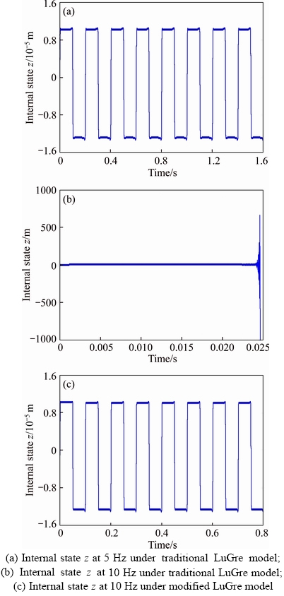
Figure 10 Observed curves of internal state z at 5 Hz and 10 Hz with 8 mm magnitude:
Another improvement of modified LuGre model is that an acceleration-dependent part Fd is added into the traditional LuGre model. According to Eq. (11), it can be seen that Fd is affected mainly by the velocity and acceleration. Fd is increased with increasing acceleration and decreasing velocity which corresponds with the characteristics of the experimental friction�Cvelocity curve. Figure 11 shows the simulated dynamic friction�Cvelocity curve at 1 Hz and 8 mm magnitude using the identified parameters obtained from IAFSA algorithm with the traditional LuGre model and modified LuGre model, respectively.
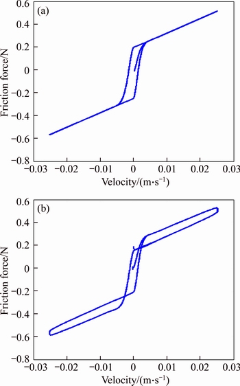
Figure 11 Simulated dynamic friction�Cvelocity curve at 1 Hz and 8 mm magnitude with traditional LuGre model (a) and simulated dynamic friction�Cvelocity curve at 1 Hz and 8 mm magnitude with modified LuGre model (b)
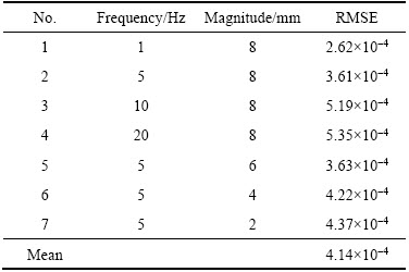
It is illustrated that the modified LuGre model is competent to depict not only the horizontal hysteresis during the presliding motion but also the vertical hysteresis during the sliding motion. However, the traditional LuGre model is only able to depict the horizontal hysteresis during the presliding motion. It is observed that the proposed modified LuGre model can describe more accurately about the essential characteristics of the dynamic friction force for electromagnetic valve actuator system. Figures 12 and 13 show the comparisons between the measured friction forces and ones simulated with the modified LuGre model at different frequencies (1, 5, 10 and 20 Hz) and a constant magnitude of 8 mm for four sinusoidal motion cycles. Figure 14 shows the comparisons between the measured friction forces and ones simulated with the modified LuGre model at different magnitudes (2, 4 and 6 mm) and a constant frequency of 5 Hz for four sinusoidal motion cycles. The root mean square errors obtained from these simulations are listed in Table 3.
The friction forces are simulated using the identified parameters obtained from IAFSA algorithm listed in Table 1 and measured data of displacement and velocity. In these figures, the blue solid line and red solid line denote the experimental data and simulated results, respectively. As can be seen from those comparison figures and the values of RMSE listed in Table 3 that the simulated results with the established mathematic friction model provide an excellent fit of the experimentally measured data. From those comparisons, it is easy to exhibit that the proposed modified LuGre model which adds ��(v) and Fdinto the traditional LuGre model is competent to capture the vertical hysteresis during the sliding regime and stabilize its discrete observer during the high-speed motions. Similarly, it also indicates that the introduction of chaotic search and Gauss mutation operator makes the IAFSA algorithm have sufficient capacity for optimizing in high-dimension space. The satisfactory match results validate the effectiveness of IAFSA algorithm for identifying both static and dynamic parameters of the proposed friction model.
It is worth mentioning that the structure of this proposed modified LuGre model can be flexible by simplifying some parameters with not sacrificing the performance of describing the friction behaviors for other specific applications. For instance, we can omit the parameters of vs, �� and make Fc equal Fs for some applications in which the value of breakaway force Fs is near to Coulomb force Fc. And the parameters of ��, �� can be omitted or predefined to specific constant to reduce the computation load for the identification.

Figure 12 Comparison (a1, a2, a3) between measured and simulated friction force with modified LuGre model at 1 Hz and magnitude of 8 mm and comparison (b1, b2, b3) between measured and simulated friction force with the modified LuGre model at 5 Hz and magnitude of 8 mm:

Figure 13 Comparison (a1, a2, a3) between measured and simulated friction force with modified LuGre model at 10 Hz and magnitude of 8 mm and comparison (b1, b2, b3) between the measured and simulated friction force with modified LuGre model at 20 Hz and magnitude of 8 mm:
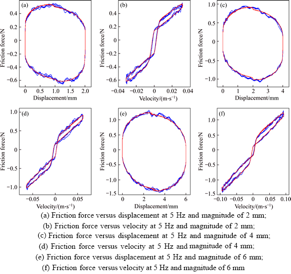
Figure 14 Comparisons between measured friction forces and ones simulated with modified LuGre model at different magnitudes (2, 4 and 6 mm) with constant frequency of 5 Hz for four sinusoidal motion cycles:
Table 3 RMSE of comparisons between measured and simulated friction forces at different frequencies and different magnitudes
6 Conclusions
1) The intrinsic practical problems of traditional LuGre friction model for real-time implementation are discussed and verified with simulation analysis.
2) A modification to the traditional LuGre friction model is made by adding an acceleration-dependent part and a nonlinear continuous switch function. It greatly enhances the capability of LuGre model for simulating the vertical hysteresis during the sliding regime and stabilizing its discrete observer for real-time digital implementation at high speeds.
3) A new IAFSA identification method which combines chaotic search and Gauss mutation operator into AFSA is presented to identify the parameters contained in the proposed modified LuGre friction model. Compared with the standard AFSA algorithm, the IAFSA algorithm increases the diversity of population to jump out of the local optimum and prompts the population to converge toward the global optimum rapidly.
4) The effectiveness of IAFSA algorithm has been validated by steady state response experiments and dynamic friction experiments. The comparisons between the measured dynamic friction forces and the ones simulated with the established mathematic friction model at different frequencies and magnitudes demonstrate that the established mathematic friction model is competent enough to describe accurately the dynamic friction characteristics existing in the electromagnetic valve actuator system.
It is worth mentioning that the presented methods for modelling and parameter identification are not limited to this mentioned application and can be transferred to many other high-speed mechanical systems.
References
[1] KAMIL M, RAHMAN M M, BAKAR R A. An integrated model for predicting engine friction losses in internal combustion engines [J]. Journal of Clinical Immunology, 2014, 4(1): 18�C22.
[2] YONG Jia-wang, GAO Feng, DING Neng-gen, HE Yu-ping. Pressure-tracking control of a novel electro-hydraulic braking system considering friction compensation [J]. Journal of Central South University, 2017, 24(8): 1909�C1921.
[3] LI Zhi-qiang, ZHOU Qing-kun, ZHANG Zhi-yong, ZHANG Lian-chao, FAN Da-peng. Prestiction friction compensation in direct-drive mechatronics systems [J]. Journal of Central South University, 2013, 20(11): 3031�C3041.
[4] de WIT C C, OLSSON H, ASTROM K J, LISCHINSKY P. A new model for control of systems with friction [J].IEEE Transactions on Automatic Control, 1995, 40(3): 419�C425.
[5] LI Zhi-qiang. LuGre-model-based friction compensation in direct-drive inertially stabilization platforms [C]// Mechatronic Systems. Hangzhou: IFAC Proceedings Volumes, 2013: 636�C642.
[6] YANG Hui, ZHAO Yan, LI Min, ZHOU Yong-jun. Study on the friction torque test and identification algorithm for gimbal axis of an inertial stabilized platform [J]. Proceedings of the Institution of Mechanical Engineers Part G: Journal of Aerospace Engineering, 2015, 303(C): 66�C79.
[7] ZHOU Xiang-yang, ZHAO Bei-lei, LIU Wei, YUE Hai-xiao, YU Rui-xia, ZHAO Yu-long. A compound scheme on parameters identification and adaptive compensation of nonlinear friction disturbance for the aerial inertially stabilized platform [J]. ISA Transactions, 2017, 67: 293�C305.
[8] FREIDOVICH L, ROBERTSSON A, SHIRIAEV A, JOHANSSON R. LuGre-model-based friction compensation [J]. IEEE Transactions on Control Systems Technology, 2010, 18(1): 194�C200.
[9] LU Lu, YAO Bin, WANG Qing-feng, CHEN Zheng. Adaptive robust control of linear motors with dynamic friction compensation using modified LuGre model [J]. Automatica, 2009, 45(12): 2890�C2896.
[10] GUO Ke-jian, ZHANG Xing-gang, LI Hong-guang, MENG Guang. Non-reversible friction modeling and identification [J]. Archive of Applied Mechanics, 2008, 78(10): 795�C809.
[11] SAHA A, WAHI P, WIERCIGROCH M, STEFASKI A. A modified LuGre friction model for an accurate prediction of friction force in the pure sliding regime [J]. International Journal of Non-Linear Mechanics, 2016, 80: 122�C131.
[12] STEFASKI A, WOJEWODA J, WIERCIGROCH M, KAPITANIAK T. Chaos caused by non-reversible dry friction [J]. Chaos, Solitons & Fractals, 2003, 16(5): 661�C664.
[13] TRAN X B, HAFIZAH N, YANADA H. Modeling of dynamic friction behaviors of hydraulic cylinders [J]. Mechatronics, 2012, 22(1): 65�C75.
[14] TRAN X B, DAO H T, TRAN K D. A new mathematical model of friction for pneumatic cylinders [J]. Proceedings of the Institution of Mechanical Engineers Part C: Journal of Mechanical Engineering Science, 2016, 230(14): 2399�C2412.
[15] LI Yi-bo, PAN Qing, HUANG Ming-hui. Model-based parameter identification of comprehensive friction behaviors for giant forging press [J]. Journal of Central South University, 2013, 20(9): 2359�C2365.
[16] TAKROURI M H. Nonlinear friction identification of a linear voice coil DC motor [D]. Sharjah: American University of Sharjah, 2015.
[17] LIN C J, YAU H T, TIAN Y C. Identification and compensation of nonlinear friction characteristics and precision control for a linear motor regime [J]. IEEE/ASME Transactions on Mechatronics, 2013, 18(4): 1385�C1396.
[18] WU Guo-qiang, RU Lai, LIU Xiang-dong. Parameters identification of valve dynamic damping system based on LuGre model and adaptive chaotic particle swarm algorithm [J]. Procedia Engineering, 2012, 29: 3732�C3736.
[19] LU Yong-zhong, YAN Dan-ping, LEVY D. Friction coefficient estimation in servo systems using neural dynamic programming inspired particle swarm search [J]. Applied Intelligence, 2015, 43(1): 1�C14.
[20] YU Yang, LI Yan-cheng, LI Jian-chun. Parameter identification and sensitivity analysis of an improved LuGre friction model for magnetorheological elastomer base isolator [J]. Meccanica, 2015, 50(11): 2691�C2707.
[21] WANG Xing-jian, WANG Shao-ping. New approach of friction identification for electro-hydraulic servo system based on evolutionary algorithm and statistical logics with experiments [J]. Journal of Mechanical Science and Technology, 2016, 30(5): 2311�C2317.
[22] CHENG Xiao-ya, JIANG Ming-yan. An improved artificial bee colony algorithm based on Gaussian mutation and chaos disturbance [C]// International Conference on Advances in Swarm Intelligence. Shenzhen: Springer-Verlag, 2012: 326�C333.
[23] NESHAT M, SEPIDNAM G, SARGOLZAEI M, TOOSI A N. Artificial fish swarm algorithm: a survey of the state-of- the-art, hybridization, combinatorial and indicative applications [J]. Artificial Intelligence Review, 2014, 42(4): 965�C997.
[24] OLSSON H. Control systems with friction [D]. Lund: Lund Institute of Technology, 1996.
[25] de WIT C C,  STR
STR M K J, SORIN M. Slides of the workshop on control of systems with friction [C]// IEEE Conference on Decision and Control. Florida, USA, 1997.
[26] LI Xiao-lei. A new intelligent optimization-artificial fish swarm algorithm [D]. Hangzhou: Zhejiang University of Zhejiang, 2003. (in Chinese)
(Edited by YANG Hua)
���ĵ���
�������ִ�л����Ķ�̬Ħ����ģ�������ʶ
ժҪ�������һ��Ӧ���ڷ������������ϵͳ�ĸĽ�LuGreĦ��ģ�ͣ��Դ�ͳ��LuGreĦ��ģ�ͽ����������������˼��ٶȷֲ��ͷ������������غ������Ľ���Ħ��ģ�ͽ���˴�ͳLuGreģ��Ӧ���ڸ�����ɢ����������ɢ�Ĺ���ȱ�ݣ�ͬʱ���������˴�ͳLuGreĦ��ģ�Ͷ���Ԥ���������ͻ�ЧӦ�������������������˶��ڻ��������ͻ�ЧӦ��Ԥ��������������������˹�����������봫ͳ�˹���Ⱥ�㷨���γ��Ż����˹���Ⱥ�㷨(IAFSA)�������ԸĽ���LuGreĦ��ģ���еIJ������б�ʶ��ͨ����̬��������Ͷ�̬Ħ��������֤��IAFSA�㷨����Ч�ԡ������������ľ�ȷĦ������ѧģ��Ԥ�����ڲ�ͬƵ�ʺͲ�ͬλ���µ�Ħ����������ʵ���Ħ���������˶Աȣ�����������Ľ���LuGreĦ��ģ���ܹ�ȷ��ģ��������ϵͳ�Ķ�̬Ħ�����ԡ�������Ľ�ģ�Ͳ�����ʶ����Ҳ��������������Ħ���ĸ��ٻ�еϵͳ��
�ؼ��ʣ�LuGreĦ��ģ�ͣ��˹���Ⱥ�㷨����˹���죻����������������ʶ���������
Foundation item: Project(2015BAG06B00) supported by the National Key Technology Research from Development Program of the Ministry of Science and Technology of China
Received date: 2017-10-11; Accepted date: 2018-06-19
Corresponding author: DU Ai-min, PhD, Associate Professor; Tel: +86-15216706918; E-mail: aimin_du@sina.com; ORCID: 0000- 0002-4196-7328
Abstract: A new modified LuGre friction model is presented for electromagnetic valve actuator system. The modification to the traditional LuGre friction model is made by adding an acceleration-dependent part and a nonlinear continuous switch function. The proposed new friction model solves the implementation problems with the traditional LuGre model at high speeds. An improved artificial fish swarm algorithm (IAFSA) method which combines the chaotic search and Gauss mutation operator into traditional artificial fish swarm algorithm is used to identify the parameters in the proposed modified LuGre friction model. The steady state response experiments and dynamic friction experiments are implemented to validate the effectiveness of IAFSA algorithm. The comparisons between the measured dynamic friction forces and the ones simulated with the established mathematic friction model at different frequencies and magnitudes demonstrate that the proposed modified LuGre friction model can give accurate simulation about the dynamic friction characteristics existing in the electromagnetic valve actuator system. The presented modelling and parameter identification methods are applicable for many other high-speed mechanical systems with friction.
