
J. Cent. South Univ. (2016) 23: 1183-1197
DOI: 10.1007/s11771-016-0368-5

MultiBoost with ENN-based ensemble fault diagnosis method and its application in complicated chemical process
XIA Chong-kun(�ij���), SU Cheng-li(�ճ���), CAO Jiang-tao(�ܽ���), LI Ping(��ƽ)
School of Information and Control Engineering, Liaoning Shihua University, Fushun 113001, China
 Central South University Press and Springer-Verlag Berlin Heidelberg 2016
Abstract:
Fault diagnosis plays an important role in complicated industrial process. It is a challenging task to detect, identify and locate faults quickly and accurately for large-scale process system. To solve the problem, a novel MultiBoost-based integrated ENN (extension neural network) fault diagnosis method is proposed. Fault data of complicated chemical process have some difficult-to-handle characteristics, such as high-dimension, non-linear and non-Gaussian distribution, so we use margin discriminant projection(MDP) algorithm to reduce dimensions and extract main features. Then, the affinity propagation (AP) clustering method is used to select core data and boundary data as training samples to reduce memory consumption and shorten learning time. Afterwards, an integrated ENN classifier based on MultiBoost strategy is constructed to identify fault types. The artificial data sets are tested to verify the effectiveness of the proposed method and make a detailed sensitivity analysis for the key parameters. Finally, a real industrial system��Tennessee Eastman (TE) process is employed to evaluate the performance of the proposed method. And the results show that the proposed method is efficient and capable to diagnose various types of faults in complicated chemical process.
Key words:
1 Introduction
Modern chemical industrial process is becoming more and more large-scale, complex, highly non-linear and highly coupled, which contributes to potential safety hazard in production process. And a simple abnormality might damage some functional portions, thus further degrade overall system, resulting in economic losses and even huge casualties. When faults occur, timely and precise detection, identification and diagnosis can lessen harmfulness, improve the safeness and reliability of the industrial system, and yet reduce losses as much as possible. Fault detection and diagnosis (FDD), as one of the key parts of computer integrated process operation system(CIPOS) in complicated industrial process, has been received wide attention from researchers all over the world.
In recent years, a lot of new fault diagnosis methods have been proposed, and some of them also have good performances, such as SDG (Signal direct graph) and its improvement [1-2], PCA (principal components analysis) and its improvement [3-5], SVM (support vector machine) and its series methods [6-7], manifold learning methods [8-9] and neural networks methods [10-11]. The SDG method, as a traditional semi-qualitative method, can cover all possible faults and find the root causes. But it costs long time, and has a high error rate and a bad real-time performance. The PCA method, as a linear dimension reduction method, can extract main variables which can describe fault reasons. However, PCA is mainly suitable for Gauss distribution fault data. SVM-series algorithms (including SVM, v-SVM, LSSVM etc) need to find very appropriate kernel function and key parameters to ensure good fault diagnosis performances. And the problem greatly limits the application of these methods. Moreover, as new features extract methods, manifold learning methods, such as FDA [12], NPE [13], MMC [14], have also been applied to fault diagnosis system. In addition, because neural network methods have strong robustness, memory ability and non-linear adaptive ability, many researchers applied them to fault diagnosis and received good results, such as ELM [15], Hopfield network [16], AANN [17] and ENN [18]. Now many scholars and experts have reached a consensus: it is very effective to diagnose faults by choosing some appropriate algorithms from the above existing fault diagnosis methods and making up new hybrid methods for complicated chemical process fault diagnosis system (CCPFDS). The new hybrid methods, such as PCA-SDG, PCA-LSSVM, LSNPE and AANN-ELM, have been proved to be successful.
As a combination of extension theory and neural network, the ENN (extension neural network) has been proved to be a novel and excellent neural network type after fuzzy neural network, genetic neural network and evolutionary neural network [19]. The ENN permits recognition and classification of problems whose features are defined over a range of values. In addition, the ENN uses a modified extension distance to measure the similarity between objects and class centers. It can quickly and stably learn to categorize input patterns and permit the adaptive processes to access significant new information. Moreover, the ENN has shorter learning time and a simpler structure than the traditional ANNs. And there have been many applications of based-ENN in the field of pattern recognition, classification and fault diagnosis [20-21]. However, the ENN��s generalization ability is not strong and when fault diagnosis data present high-dimension and highly non-linear, the ENN does not perform well.
Due to its advantage in improving the generalization ability of the learning system, ensemble learning [22] is rapidly growing and attracting more and more attention for fault diagnosis, pattern recognition and other various domains over the past two decades. MultiBoost (MB), as a fusion of Wagging and Ada Boost (Adaptive boosting algorithm), has been proved to be an excellent ensemble learning algorithm [23-24]. MB can effectively reduce the classification model bias and variance by adding the weighting mechanism of Wagging in classifiers of AdaBoost. So, we use ENN as a base classifier unit, and build an integrated ENN classifier based on Multiboost strategy. In addition, pre-processing of fault data is also a very important work in CCPFDS. Due to high dimension of chemical process, we employ margin discriminant projection (MDP) [25] algorithm to reduce dimensions and extract main features. MDP is a novel supervised linear dimension reduction algorithm, aims to minimize the maximum distance of samples belonging to the same class and maximize the minimum distance of samples belonging to different classes, and at the same time preserve the geometrical structure of data manifold. Compared with other feature extraction algorithms, such as PCA, FDA, MMC, MDP is good at preserving the global properties, such as geometrical and discriminant structure of data manifold, and can overcome small size sample problem. Besides, affinity propagation (AP) [26-27] clustering algorithm was used to select core data and boundary data with training samples to eliminate redundant information of fault data and reduce memory consumption and shorten learning times. Thus, to improve the ENN��s performance on fault diagnosis, we propose a MultiBoost-ENN ensemble fault diagnosis method based on margin discriminant projection and affinity propagation (MDPAP-MBENN). Finally, some artificial data sets and the real chemical industrial process-TE process are tested to prove the validity of the proposed method.
2 ENN classifier
The ENN is a combination of neural networks and the extension theory [19]. It provides a new distance measurement for the classification process, and embeds the salient features of parallel computation power and learning capability. The schematic structure of ENN is depicted in Fig. 1. It comprises both the input layer and the output layer. In the network, there are two connection values (weights) between input nodes and output nodes; one connection represents the lower bound for the classical domain of the features, and the other connection represents the upper bound. The connections (weights) between the j-th input node and the k-th output node are ��L and ��U. The output layer is a competitive layer.
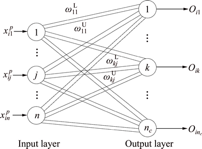
Fig. 1 Structure of ENN
ENN uses extension distance (ED) to measure similarities between the tested data and the class centers. ED is presented below:
 (1)
(1)
where 
In Fig. 2, the ED can be used to describe the distance between a point x and a range  . And Fig. 2 also shows that the rate of ED change is inversely proportional to the length of the range. The shorter thelength of the domain is, the larger the extension distance variation is. When the length of the range is very short, a little position change of the point x can lead to a very big change of the ED value. Therefore, compared with the nonlinear mapping of the methods such as BP (i.e. back propagation network), the ED caneasily identify the difference between the features of the training samples by the extension theory space mapping. Due to its advantages, the ED can make the structure of the ENN clear and stable, which is a significant advantage in classification.
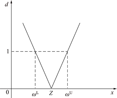
Fig. 2 Extension distance
The learning of the ENN can be seen as a supervised learning process. The purpose of learning is to tune the weights of the ENN to achieve good classification performance or to minimize the classification error. The major steps of learning algorithm can be described as follows.
Let the training data set be X={X1, X2, ��, where Np is the total number of training instances. The i-th instance in training data set is
 where n is the total number of the feature of instances, and p denotes the category of the i-th instance. To evaluate the ENN performance, the error rate function E is defined below:
 (2)
(2)
where n is the total error number. The detailed supervised learning algorithm can be described as follows.
First of all, set the initial weights  and class center zkj, and build the matter-element model of extension theory:
 k=1, 2, ��, n (3)
Then, use the ED to calculate the distance between the training instance  and the k-th class:

k=1, 2, ��, nc (4)
where 
Find k*, such that  If k*=p, then input the next training instance and calculate the extension distance; otherwise, update the weights of the p-th and the k*-th classes as Eq. (5)-(10). Repeat the above steps until the training process has converged, or the total error E has arrived at a preset value.
1) Update the center of the p-th and the k*-th cluster:
 (5)
(5)
 (6)
(6)
2) Update the weights of the p-th and the k*-th cluster:
 (7)
(7)
 (8)
(8)
 (9)
(9)
 (10)
(10)
where �� is a learning rate. The result of tuning the weights of two classes is shown in Fig. 3. And Fig. 3 clearly indicates the change of the EDA and EDB. The category of instance xij is changed from class A to B due to EDA<>B. From this step, it can be clearly seen that the learning process is only to adjust the weights of the p-th and the k*-th class. Therefore, the proposed methodhas a speed advantage over the other supervised learning algorithms, and can quickly adapt to new and important information.
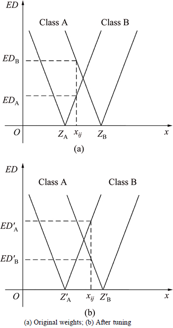
Fig. 3 Results of tuning weights:
3 MuliBoost with ENN-based ensemble classification method
Identifying various faults accurately is the key component of fault diagnosis system. Fault data of complicated chemical process always contain some useless feature vectors and redundant information, and can cause much memory consumption and low fault recognition rate. Hence, extracting the appropriate features and selecting the key samples are very important for improving the recognition ability of ensemble neural network classifier.
3.1 Feature extraction
Feature selection has been proven to be an effective means when dealing with large dimensionality which contains many irrelevant features [28]. Margin discriminant projection (MDP) is a novel supervised linear dimension reduction algorithm. Compared with other feature extraction algorithms, such as PCA, FDA and MMC, MDP is good at preserving the global properties, such as geometrical and discriminant structure of data manifold, and can overcome small size sample problem. Therefore, we use MDP to reduce dimension and extract main feature vectors. The concept about dimension reduction is defined as follows.
Definition 1: Let the input data set be X and output data set be Y. If there is an explicit mapping relationship between X and Y, it can be presented below:
 (11)
(11)
where V is the projection matrix.
To keep the whole geometry structure of data sets, the orthogonal constraint VTV=I is introduced into the process. The objective function of MDP can be expressed as follows:
 (12)
(12)
where ��(ci, cj) and ��(ci) are respectively the distance of two samples (ci and cj) that belong to the different classes and the distance of samples (cj) that belong to the same class in the dimension-reduced feature space. The distance of low-dimensional samples after projection is depicted as follows:
 (13)
(13)
Besides, the distance of samples belongs to the different class and the distance of samples belongs to the same class are also described as follows:
 (14)
(14)
 (15)
(15)
Equations (13)-(15) is plugged into Eq. (12), and then, the objective function can be transformed into
 (16)
(16)
To calculate the objective function (Eq. (16)) easily, a method called graph embedding is used. Thus, inter class similarity weight W(b) and within class similarity weight W(w) is defined below:
 (17)
(17)
 (18)
(18)
Therefore, the objective function (Eq. (16)) can be depicted as follows:
 (19)
(19)
According to the conclusion of margin fisher analysis in Ref. [29], we can find that:

 (20)
(20)
Thus, with a combination of Eq. (19) and Eq. (20), objective function can be depicted as follows:
 (21)
(21)
where 
 L(b) and L(w) are Laplacian matrix.
To calculate optimal projection matrix V, the incomplete Cholesky decomposition method (from Ref. [30]) is applied to Eq. (20). Then, output data set Y can be calculated by using Eq. (11).
3.2 Sample selection
In the learning of ensemble classifier, training samples occupies a very important position. There are always many similar, repetition and noise samples among training samples. Therefore, we use the improving semi-supervised affinity propagation (AP) algorithm to find class center of each type of fault and select ��key�� samples by defining new rules.
The basic semi-supervised AP is a fast, effective clustering method. The basic idea of AP clustering theory is to calculate the similarity matrix SN��N among the data points whose number is N. And every sample point was viewed as a potential cluster center. Moreover, s(k,k) which is a diagonal element in the SN��N is regarded as the evaluation standard of a cluster center k. The larger the value s(k,k) is, the greater the possibility of becoming a clustering center is. And this value s(k,k) is also called tendency parameter ��. Then, the degree of attraction and the degree of membership are updated constantly for every point to generate a plurality of high quality clustering centers and to distribute the rest points into the corresponding clustering labels. The degree of attraction and the degree of membership among these sample points is defined as follows:
Definition 2: The degree of attraction r(i,k) is used to describe the suitable degree whether the point k is used as the cluster center i or not.
Definition 3: The degree of membership a(i,k) is used to describe the suitable degree whether the point i is used as the cluster center k or not.
To find the right cluster center xk, AP algorithm keeps iterating for r(i,k) and a(i,k):
 (22)
(22)
 (23)
(23)
where �� is damping coefficient and it is used to adjust the iterative update speed. The larger the value of r(i,k) or a(i,k) is, the greater the possibility whether the point k becomes a clustering center or not, and whether the point i is used as the cluster center k or not is.
The semi-supervised strategy of AP is the pairwise constraints by using prior information to adjust the similarity matrix. The pairwise constraints can be divided into two types: Must-link, the two points must belong to the same class, that is the sets M={(xi, xj)}; Cannot-link, restrictions between two points are not in the same class, that is the sets C={(xi, xj)}. Therefore, the constraint adjustment rules of semi-supervised strategy are as follows:
1) If  then s(i,j)=s(j,i)=0 (24)
2) If  then s(i,j)=s(j,i)=-�� (25)
3) If  then s(i,j)=s(j,i)= max{s(i,j), s(i,k)+s(k,j)} (26)
4) If  M, then s(i,j)=s(j,i)=-�� (27)
However, the AP has a poor performance when the inner structure of data is very complex. From the study of manifold learning, we find that manifold distance has been demonstrated to reflect the distance faithfully between points from the viewpoint of data structure. Therefore, we use the manifold distance as a measure of matrices similarity instead of euclidean distance.
The calculation method of manifold distance is given as below:
1) For the k neighborhood and the k anti- neighborhood in the set X, the adjacency graph G=(V, E) is constructed on the manifold M. If  then the vector eij is the euclidean distance between the two points dX(xi, xj); otherwise, eij=��.
2) To obtain the approximate geodesic distance matrix DG={dG(xi, xj)}, the shortest path dG(xi, xj) in the adjacency graph G=(V, E) and the geodesic distance dM(xi, xj) on the manifold M are calculated. Let Pij as the sets which contain all paths between xi and xj in G. Then,
 (28)
(28)
Calculate the manifold distance between arbitrary two nodes in G.
 (29)
(29)
Then, similarity degree between xi and xj is described as follows:
 (30)
(30)
where �� is the Gauss nuclear radius.
To select key samples (i.e. core samples and boundary samples) as training samples, we divide the original samples into core points, boundary points and noise points by neighborhood density index. The core samples and boundary samples are used as the training data. The definition of selecting rules are given as follows:
Definition 4: Neighborhood density index:
 (31)
(31)
where V��(x) is the ��-neighborhood of the class center x (x is the class center of every fault), and V��(x) is ��-anti-neighborhood of the class center x.
Definition 5: Core point, boundary point, noise point. If ��(k,x)��0.5, then x is a core point; If �ơܦ�(k,x)<0.5, where �� is arbitrarily small positive, then x is a boundary point; If ��(k,x)<��, then x is a noise points.
The above selection method can quickly and accurately eliminate the non-representative and useless samples around these centers of fault data. Obviously, the selection operation can effectively reduce the computation and improve the execution speed of fault diagnosis.
3.3 Ensemble ENN classifier based on MultiBoost strategy
3.3.1 MultiBoost-based ENN ensemble classifier
In the Bagging algorithm [31], data set can be described as If T base classifiers (Ct, t=1, 2, ��, T) are integrated, we can use the classification results of Bootstrap algorithm to vote and make decisions:
 (32)
(32)
where  is the indicator function.
Compared with the Boostrasp sampling method of Bagging strategy, Wagging gives specified weight to every training instance by obeying continuous Poisson distribution. The calculating formula of weights is shown as
 (33)
(33)
However, unlike the direct T times iterations of the Adaboost algorithm, the MultiBoost (MB) strategy defines some sub-decision groups and a mark variable Ii (i=1, 2, ��, ��) which can confirm iteration times of sub- decision group. In the MB strategy, the i-th sub-decision group contains Ii base-classifiers constructed by the AdaBoost. And the whole sub-decision groups need to be combined by the Wagging strategy. The value of Ii usually follows rules:
 (34)
(34)
In addition, whether the error caused by sub-decision group is too high or not in every iteration process, the next sub-decision group will keep on with iteration and the iteration terminated times will be increased. If the classification error of last sub-decision group is too high or too low, the algorithm will use one or more extra sub-decision groups until the error fulfills the requirement.
The data set can be described as follows:  , and the weight value of every sample can be set to 1. And it will produce new data set S��. When every sub-decision group��s iteration is end, the weights of S�� will be reset and normalized with continuous Poisson distribution, and then the next sub- decision group��s iteration will be continued. In every iteration process of the base classifier, the base classifier error ��t (t=1, 2, ��, T) can be calculated as follows:
 (35)
(35)
The weights of base-classifiers to final combination classification model are ��t, t=1, 2, ��, T. Because the value of ��t is different for every iteration, we can divide it into three situations:
1) If ��t>0.5, then ignore the classifier and let training data set be reset and normalized by obeying continuous Poisson distribution, and start to analyze the next sub- decision group till ��t��0.5.
2) If ��t=0, then set ��t=10-10, and repeat the above process.
3) If 0<��t��0.5, then set ��t=��t/(1-��t). For every sample of S��, the weights of wrong classification samples are multiplied by 2��t and the weights of right classification samples are multiplied by 2(1-��t), and the smallest weight is 10-8. In a word, the classification function can be described as follows:
 (36)
(36)
The above ensemble strategy establishes a decision system which can ensure that the sub-ENN classifiers are running correctly. Figure 4 shows the basal structure of multiple ENN ensembles network. The sub-ENNmn is the m-th classifier of the n-th layer network. In this ensemble classifier, every sub-ENN classifier, which is used as a simple and independent unit, can fully exert the advantages of ENN.
Given the above, we propose a novel classification algorithm based on MDPAP-MBENN. The proposed classification algorithm is described as follows. And among this algorithm, k is the auxiliary variable and its initial value is 1.
Step 1: Set the dimension r of dimension-reduced feature space and extract main features.
Step 2: Select samples using the improving semi- supervised AP algorithm and build the training set S.
Step 3: Build the matter-element model of extension theory and calculate every element weight of S by Eq. (3)-(10). Then the new training set is S��.
Step 4: For t=1, 2, ��, T.
Step 4.1: Calculate Ii by Eq. (36) and if Ik=t, then make training data be reset and normalized randomly to obey continuous Poisson distribution; k++.
Step 4.2: Use ENN base-classifier to classify fault type, and  .
.

Fig. 4 Graph of multiple ENN ensembles
Step 4.3: Calculate the fault identification rate ��t by Eq. (35). And the weights of base-classifiers to output ensemble classifier model are ��t.
Because the value of ��t is different for every iteration process, we can divide it into three situations:
1) If ��t>0.5, then make training data be reset and normalized randomly to obey continuous Poisson distribution; k++; Go to Step 4.2.
2) If ��t=0, then make training data be reset and normalized randomly to obey continuous Poisson distribution; k++.
3) If 0<��t��0.5, then set ��t=��t/(1-��t) and update the every sample weights of S��. For the right classification samples, Weight(xj)=weight(xj)/2(1-��t). For the wrong classification samples, Weight(xj)=weight(xj)/2��t,
3.3.2 Mathematical analysis of generalization error
To verify the feasibility of the proposed MultiBoost ENN ensemble classifier (MBENN), the mathematical derivation and proof of generalization error are given below.
Suppose the data set D is composed of N instances ({[x(1), d(1)], [x(2), d(2)], ��, [x(N), d(N)]}), and the MBENN ensemble F is composed of M sub-ENN classifier (f1, f2, ��, fM). In Ref.[32], KROGH was given the generalization error formula of integrated method:
 (37)
(37)
where  is the error of sub classifiers and
  is the different degree among the sub classifiers.
If the integrated rule of the MBENN obeys simple averaging method, we can find:


 (38)
(38)
Hence we can deduce that:


 (39)
(39)
In Eq. (39), the first polynomial is the i-th sub- ENN generalization error and the second polynomial is the error correlation Ci between the i-th sub-ENN and other sub-ENNs.
 (40)
(40)
So, the integrated error of the MBENN is shown below:
 (41)
(41)
where Ji is the error rule function of the j-th sub-ENN.
From Eq. (41), we can find that E can reach the minimum by minimizing the error rule function Ji.Besides, as long as Ci meets the requirement ,the generalization error of the MBENN classifier will be less than the average error of a single sub-ENN classifier. And it also indicates that the MBENN is a more competitive classification tool than a single ENN.
4 Simulation and analysis
Fault identification is a very important component for fault diagnosis system in complicated chemical process. And it is also exactly the focus of the proposed MDPAP-MBENN algorithm. To verify the effectiveness of this identification method, four benchmark data sets which are similar to fault data are selected and tested on the platform of MATLAB 2014a. Then we make a detailed sensitivity analysis for the key parameters on the basis of the above simulation. And one of the main goals of the simulation is providing some reference suggestions and experiences for parameters selection of the next application. Besides, an evaluation index called Fowlkes and Mallows index (FMI) is used to accurately evaluate the classification performance of the identification tool.
4.1 Evaluation index
Compared with conventional evaluation indexes about classification, such as accuracy rate, error rate, the FMI has been proved to be a novel and effective classification performance evaluation function in Ref. [33].
Let input set and output set be C={C1, C2, ��, Ck} and C��={C��1, C��2, ��, C��k}. The classification index F of the FMI is defined as follows:
 (42)
(42)
where a is a set belonging to the same category in C and C��; b is a set belonging to the same category in C and the different category in C��; and C is a set belonging to the different category in C and the same category in C��.
4.2 Simulation and discussion
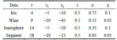
In this work, the four data sets are Iris data set (from UCI), Wine data set (from UCI), Ionosphere data set (from UCI) and Segment data set (from LIBSVM). The detailed tested data sets are listed in Table 1. To ensure the execution of the experiments, we must set some key parameters, such as dimension-reduced r, tendency parameter ��1 and ��2 in cluster analysis, damping coefficient ��, Gauss nuclear radius �� and learning rate ��. Among them, tendency parameter ��2 for sample selection process can be obtained by iterating. The other parameters can be set by experience of experts and cross validation method. The detailed information of parameters are listed in Table 2.
Table 1 Attributes of tested data
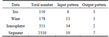
Table 2 Information of key parameters
The 10-fold cross validation method is used to ensure the validity and fairness of this experiment. Firstly, every set-tested can be randomly divided into ten almost equal parts. Secondly, the system chooses nine parts as the training data set, and lets the rest of the parts as the testing data set. To be more objective, each method are done 10 times and the average results are used as an evaluation index for comparison.
In this work, the ENN and the MBSVM are used as the contrast tests by the same ways. The parameters of the MBSVM can be set by Ref. [7]. Tr, Te and F respectively represent the average value of training precision, accuracy rate and evaluation index. Tepoch represents training time.
Table 3 shows the comparison results of training performance of the above three methods. From Table 3, it can be seen that the three methods all have a good learning performance for Iris classification problem. Besides, for data sets, such as Wine, Ionosphere and Segment, we can also find that the proposed MDPAP- MBENN has shorter learning time, higher training accuracy rates than other methods. Especially for high- dimension data sets, such as Ionosphere and Segment, the proposed MDPAP-MBENN has the better training performance. Table 4 shows the comparison results of recognition performance of various methods. In this experiment of high-dimension data classification problems, such as Ionosphere and Segment, the accuracy rates of the MDPAP-MBENN have reached 93.9% and 92.6%. From the above, the results indicate that the MDPAP-MBENN is effective, and it has a shorter learning time and a higher classification accuracy than the ENN and the MBSVM.
Table 3 Comparison of training performance
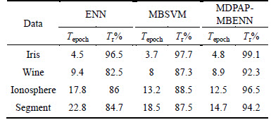
Table 4 Comparison of recognition performance

4.3 Sensitivity analysis of parameters
The key parameters of the proposed MDPAP- MBENN need to be set to ensure an accurate and stable classification ability. The parameters involve r, ��1, ��2, ��, �� and ��. Because the parameters ��1, ��2, ��, �� have been discussed in Ref. [26-27, 33], this work mainly discusses the influence of the parameters r and �� for the MDPAP-MBENN.
Figure 5 shows the impact curves of the dimension- reduced parameter r on classification performance. In Fig. 5, the solid line and dotted line respectively represent the test accuracy rate Te and performance index F. From Fig. 5, it can be seen that the dimension-reduced parameter r has a great effect on classification ability. Iris data set whose dimension is four is low-dimension data. It is clear that the MDPAP- MBENN has a good identification performance when r is 4. It indicates that the dimension-reduction operation of the proposed method is not necessary for the low- dimensional data.
From UCI, we can find that the spatial distribution structure of Wine is very complicated. So, most of its features contain key information that decide the structure of Wine, so its features should be remained as many as possible.
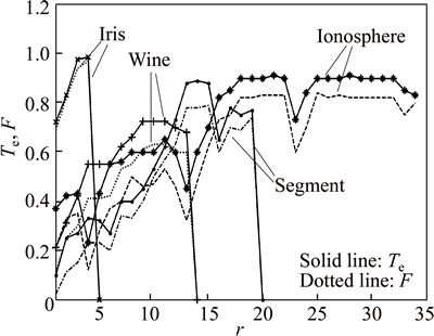
Fig. 5 Impact of r on identification performance
High-dimensional and large-scale data sets, such as Ionosphere and Segment, contain a lot of redundant information which needs to be eliminated. Figure 5 shows that it has a great performance for Ionosphere set with r=21 and Segment set with r=14. It also indicates that the operation of feature extraction can improve the classification performance for high-dimensional and large-scale data sets. Besides, the curve of the index F and the curve of the accuracy rate Te have almost the same trend in Fig. 5. It indicates that the F is suitable to evaluate the classification ability of the proposed MDPAP-MBENN. Figure 6 shows the curve relating learning rate �� to training speed. The abscissa of Fig. 6 is the training steps of the MDPAP-MBENN.
From Fig. 6, it can be seen that the learning rate �� has a great influence on the training speed of the proposed method. Because the value of �� ranges from 0 to 0.2, it is clear to easily obtain an appropriate value by some simple experiments. Moreover, it indicates that the MADAP-MBENN permits fast adaptive process for significant and new information and it is easy to acquire knowledge and maintain the classification database.
5 Fault diagnosis based on MDPAP-MBENN and its application
5.1 Fault diagnosis system
The system framework of the proposed MDPAP- MBENN fault diagnosis method is depicted in Fig. 7. The fault diagnosis system contains the core ensemble classifier module and other peripheral modules. The ENN is selected as base-classifier to build core module. The MDP is used as main feature extraction module and the AP is used to build other sample selection module.
The state data in the historical sample database can be used as training samples and be input in the base- classifiers by using continuous Poisson distribution sampling mechanism in each iteration process. Then the MB strategy is applied to the base-classifiers ensemble process to obtain a better classification results.
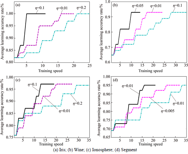
Fig. 6 Relationship between learning rate �� and training speed:
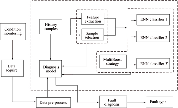
Fig. 7 Fault diagnosis system based on MDPAP-MBENN
In CCPFDS, we need to build the peripheral system module part. The system state monitoring module is a real-time monitoring system. It can collect and pre- process the system state data at intervals, and then those data will be input in the core ensemble classifier module to fault diagnosis and identification. The data are acquired by a certain time interval. If fault occurs, the system will automatically identify and confirm its fault type to provide a strong basis for next step-solve it.
5.2 Application of TE challenge process
To demonstrate the feasibility and effectiveness of MDPAP-MBENN method, we apply it to fault diagnosis for Tennessee Eastman (TE) process. In this section, five methods are employed for fault diagnosis separately: KPCA (T2), KPCA(SPE), MBSVM, ENN and MDPAP- MBENN. The purpose is to show the performance of different methods, and to verify the advantages of the proposed method.
5.2.1 TE process
TE process is a realistic challenging complicated chemical industrial process to evaluate process control, process monitoring and diagnostic methods. The flowchart of TE process is shown in Fig. 8. There are five major operating units in this process: (1) reactor, (2) condenser, (3) recycle compressor, (4) vapor/liquid separator, (5) product stripper. The process contains 41 measured variables and 12 manipulated variables. The 12th manipulated variable, which is the agitator speed of the reactor stirrer, is not used in the controller structure. And it is not changed during the course of operation of the plant. Therefore, the symptom input vector of the fault diagnostic scheme has 52 components consisting of 22 continuous process measurements, 19 composition measurements, and 11 manipulated variables.
The reactor product stream passes through a condenser and arrives at a vapor-liquid separator. Non- condensed components are recycled back through a centrifugal compressor to the reactor feed. Condensed components move to a product stripping column to remove the remaining reactant with feed stream. Products G and H exit the stripper base and they are separated in a downstream refining section which is not included in the problem. Within the mixing zone, all feed streams and the recycle streams are mixed and fed into the reactor. The excessive heat is removed by cooling water. Feed and product streams are in the vapor phase.
There are four main reactions in this process. Four reactants react to produce two products, and an inert and a by-product are produced along with the reaction. The chemical reactions are irreversible ones and of release heat. At the same time, the process consists of eight components: A, B, C, D, E, F, G, and H. Among these components, gaseous reactants A, C, D, E and inert component B are sent into the reactor, liquid component G and H are produced after the reaction reacted. Substance F is the by-product. The four reactions are depicted as follows:
A(g)+C(g)+D(g)��G(l) (product 1)
A(g)+C(g)+E(g)��H(l) (product 2)
A(g)+E(g)��F(l) (by-product)
3D(g)��2F(l) (by-product)
5.2.2 Discussion and analysis
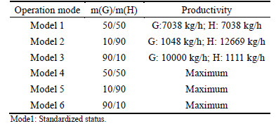
The TE simulation contains 21 pre-programmed faults which is listed in Table 5. Sixteen of these faults are known and five are unknown. In addition, due to the difference of G/H mass ratio, the process is divided into six operation modes. The modes are shown in Table 6. In this study, we select mode 1( is standardized status mode) as the operation mode of the whole experiment. The sampling interval to collect the simulated data for the training and testing sets is 3 min.
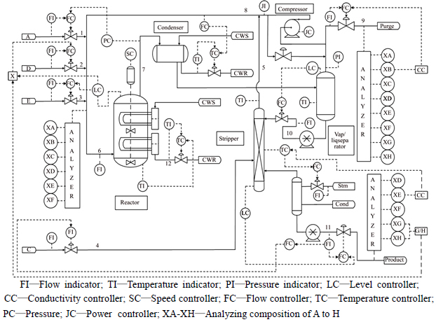
Fig. 8 Flowchart of TE process:
Table 5 Process disturbance in TE process
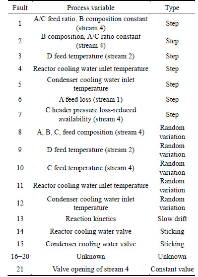
Table 6 Operation modes of TE process
In the process of generating training samples, the simulation started with no faults, and the faults were introduced one simulation hour into the run. The total number of observations generated for each run was 500, but only 480 observations were collected after the introduction of the fault. Therefore, the training samples for each fault contain 20 normal samples and 480 fault samples. In the process of generating training samples, all faults in the data set are introduced from the 160-th sample and all the data are scaled prior to the application. Faults began in the first beginning of 9 h, that is to say, faults are introduced ever since the 161-th sample. The simulation time is 48 h. The test samples contain 160 normal samples and 800 fault samples.
For the KPCA-based fault diagnosis method, we use the Gaussian kernel function as the kernel function and the kernel parameter value is 400, and the number of the kernel vectors is 38 according to experience. The parameters of the ENN and the MBSVM can be configured in accordance with Ref. [19] and Ref. [7], respectively. The parameters of the proposed MADPAP- MBENN have been discussed in the above section, and the feature vectors can be set to 27(r=27).
As a main comparative approach, the KPCA method is a typical fault diagnosis method based on the statistic strategy. And it has been widely used in the application of CCPFDS. But as a statistics-based method, it is a challenging work to identify every types of faults. However, the neural network-based fault diagnosis method has strong generalization ability and nonlinear mapping ability so that it is competent to this task.
Tables 7 and 8 respectively show the false detection rates and miss detection rate of the 21 faults using the MDPAP-MBENN in the TE process. From Table 7, we can find that the false detection rates of KPCA (T2), KPCA (SPE), MBSVM and MDPAP-MBENN are obviously lower than the ENN. And it indicates that the single ENN is not suitable for complicated chemical process. Moreover, the false detection rate of the MDPAP-MBENN is lower than that of KPCA (T2), KPCA (SPE) or MBSVM. It indicates that the proposed method has a better performance for identifying faults than other methods.
Table 7 False detection rates of 21 faults in TE process(%)
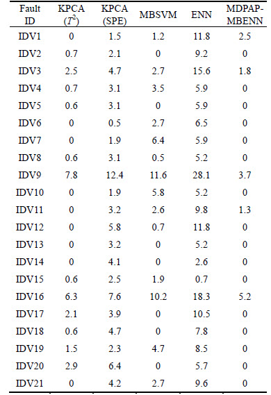
Table 8 Miss detection rates of 21 faults in TE process(%)
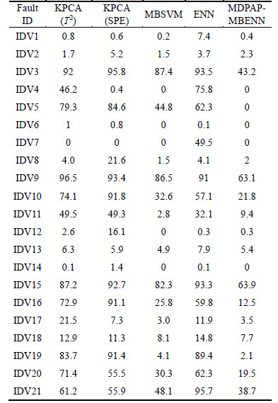
When fault 3, fault 9 and fault 15 occur, the process data change is very little, and the mean error or the variable barely gets affected. And this change will lead to the high false detection rates of the data statistics-based fault diagnosis methods. Hence, in Table 8 we can find that the miss detection rates of fault 3, fault 9 and fault 15 are higher than other faults, and KPCA(T2) and KPCA(SPE) are not good at identifying these three types of faults. However, due to the strong generalization ability and nonlinear mapping ability, the MDPAP- MBENN has a good performance than other methods. Besides, when the large-amplitude faults occur, such as fault 1, fault 2, fault12, fault 13 and fault 14, KPCA (T2), KPCA (SPE), MBSVM and MDPAP-MBENN have higher false detection rates but ENN. In addition, the performance of the proposed method is obviously superior to other method from Tables 7 and 8.
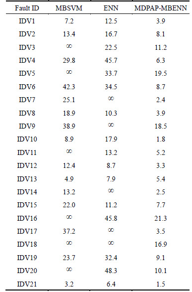
In addition, the detection and identification time of the above methods are also very important for the fault diagnosis system in the chemical process. So, we conduct multiple tests and use the average of fault diagnosis time as a comparison. Table 9 shows the fault diagnosis time of the MBSVM, ENN and MDPAP-ENN for every type of fault.
From Table 9, we can find that the MBSVM and the single ENN do not effectively identify the types of unknown faults, such as fault15-fault19. And the MBSVM has a worse performance than the ENN. It also indicates the generalization ability of the MBSVM is not strong for fault diagnosis process. Besides, compared with the single ENN, the MDPAP-MBENN can identify various types of faults faster, and especially for the unknown types of faults it has a shorter diagnosis time. The results demonstrate that the proposed method has a better adaptive process for some unknown fault information.
Table 9 Comparative analysis of fault diagnosis time of 5 fault miss detection rates of 21 faults in TE process (s)
6 Conclusions
1) To improve the ability of single ENN classifier, we propose a novel MultiBoost integrated ENN classifier based on margin discriminant projection and affinity propagation (MDPAP-MBENN) for fault diagnosis of complicated chemical processes. The proposed method consists of three parts: feature extraction, sample selection and ensemble classifier. The proposed method not only has a good classification ability but also keeps the advantage of the single ENN: it permits an adaptive process for significant and new information. And this strength is very useful for identifying the new types of faults in complicated chemical process.
2) In addition, with the strong generalization ability and nonlinear mapping ability, the MDPAP-MBENN has a better performance than KPCA, MBSVM and a single ENN in the application of CCPFDS. The proposed method can identify new types of faults but it cannot diagnose several faults at the same time. For the moment, if several faults happen at the same time, the procedure assigns the observation to only one class. An outlook of interest would be to define a threshold so that new data can be assigned to more than one class if the values of output neurons exceed the threshold. The main cause of function in the proposed diagnostic scheme is related to the supervisor agent. Therefore, another field of interests would be the use of other advanced techniques as supervisor agent for triggering the right local ENN classifier. Further work will focus on complicated nonlinear chemical process to see the effectiveness of related approaches.
References
[1] GAO Dong, WU Chong-guang, ZHANG Bei-ke, MA Xin. Signed directed graph and qualitative trend analysis based fault diagnosis in chemical industry [J]. Chinese Journal of Chemical Engineering, 2010, 18(2): 265-276.
[2] MAURYA M R, RENGASWAMY R. Application of signed digraphs-based analysis for fault diagnosis of chemical process flowsheets [J]. Engineering Application of Artificial Intelligence, 2004, 17(5): 501-518.
[3] LAU C K, GHOSH K, HUSSAIN M A, CHE HASSAN C R. Fault diagnosis of Tennessee Eastman process with multi-scale PCA and ANFIS [J]. Chemometrics and Intelligent Laboratory, 2013, 120: 1-14.
[4] YU Jie. A support vector clustering-based probabilistic method for unsupervised fault detection and classification of complex chemical processes using unlabeled data [J]. AIChE Journal, 2013, 59(2): 407-419.
[5] JIANG Qing-chao, YAN Xue-feng. Just-in-time reorganized PCA integrated with SVDD for chemical process monitoring [J]. AIChE Journal, 2014, 60(3): 949-965.
[6] WANG Xian-fang, WANG Sui-hua, DU Hao-ze, WANG Ping. Fault diagnosis of chemical industry process based on FRS and SVM [J]. Control and Decision, 2015, 30(2): 353-356. (in Chinese)
[7] LU Feng, LI Xiang, DU Wen-xia. MultiBoost with SVM-based ensemble classification method and application [J]. Control and Decision, 2015, 30(1): 81-85. (in Chinese)
[8] CHEN Xin-yi, YAN Xue-feng. Fault diagnosis in chemical process based on self-organizing map integrated with fisher discriminant analysis [J]. Chemical Journal of Chemical Engineering, 2013, 21(4): 382-387.
[9] SONG Bing, MA Yu-xin, FANG Yong-feng, SHI Hong-bo. Fault detection for chemical process based on LSNPE method [J]. Chinese Journal of Chemical Engineering Journal, 2014, 65(2): 620-627. (in Chinese)
[10] ZHOU Yu, PEDRYCZ W, QIAN Xu. Application of extension neural network to safety status pattern recognition of coal mines [J]. Joumal of Central South University of Technology, 2011, 18: 633-641.
[11] BARAKAT M, DRUAUX F, LEFEBVRE D, KHALIL M, MUSTAPHA O. Self adaptive growing neural network classifier for faults detection and diagnosis [J]. Neurocomputing, 2011, 74: 3865-3876.
[12] ZHU Zhi-bo, SONG Zhi-huan. A novel fault diagnosis system using pattern classification on kernel FDA subspace [J]. Expert System with Application, 2011, 38(6): 6895-6905.
[13] JIANG Qing-chao, YAN Xue-feng. Probabilistic weighted NPE-SVDD for chemical process monitoring [J]. Control Engineering Practice, 2014, 28: 74-89.
[14] LI Xiao-qian, SONG Qiang, LIU Wen-hua, RAO Hong, XU Shu-kai, LI Li-cheng. Protection of nonpermanent faults on DC overhead lines in MMC-based HVDC systems [J]. IEEE Trans on Power Delivery, 2013, 28(1): 483-490.
[15] GAO Hui-hui, HE Yan-li, ZHU Qun-xiong. Research and chemical application of data attributes decomposition based hierarchical ELM neural network [J]. Chinese Journal of Chemical Engineering, 2013, 64(12): 4348-4353. (in Chinese)
[16] HE Ding, ZHANG Jin-song. Fault strategy of time delay analysis based on Hopfield network [J]. Chinese Journal of Chemical Engineering, 2013, 64(2): 633-640. (in Chinese)
[17] PENG Di, HE Yan-lin, XU Yan, ZHU Qun-xiong. Research and chemical application of data feature extraction based AANN-ELM neural network [J]. CIESC Journal, 2012, 63(9): 2920-2925. (in Chinese)
[18] WANG Meng-hui. Partial discharge pattern recognition of current transformers using an ENN [J]. IEEE Trans on Power Delivery, 2005, 20(3): 1984-1990.
[19] WANG Meng-hui, HUNG C P, Extension neural network and its applications [J]. Neural Networks, 2003, 16(5): 779-784��
[20] CHAO K H, WANG M H, HSH C C. A novel residual capacity estimation method based on extension neural network for lead-acid batteries [J]. Lecture Notes in Computer Science, 2007, 4493: 1145-1154.
[21] CHAO K H, LEE R H, WANG M H. An intelligent traffic light control based on extension neural network [J]. Lecture Notes in Computer Science, 2008, 5177: 17-24.
[22] TANG Sheng, ZHENG Yan-tao, WANG Yu, CHUA Tat-seng. Sparse ensemble learning for concept detection [J]. IEEE Trans on Multimedia, 2012, 14(1): 43-54.
[23] SHEN Chun-hua, HAO Zhi-hui. A direct formulation for totally- corrective multi-class boosting [C]// Computer Vision and Pattern Recognition (CVPR) of 2011 IEEE Conference. Washington D.C.: IEEE Computer Society, 2011: 2585-2592.
[24] DJALEL B, ROBERT B F, NORMAN C, COLIN F D, BALAZS K. MultiBoost: A multi-purpose boosting package [J]. The Journal of Machine Learning Research, 2012, 13(1): 549-553.
[25] HE Jin-rong, DING Li-xin, LI Zhao-kui, HU Qing-hui. Margin discriminant projection for dimensionality reduction [J]. Journal of Software, 2014, 25(4): 826-838. (in Chinese)
[26] SHANG F H, JIAO L C, SHI J R, WANG F, GONG M G. Fast affinity propagation clustering: A multilevel approach [J]. Pattern Recognition, 2012, 45(1): 474-486.
[27] WANG Chang-dong, LAI Jian-huang, SUEN Ching Y, ZHU Jun-yong. Multi-exemplar affinity propagation [J]. Pattern Analysis and Machine, 2013, 35(9): 2223-2237.
[28] LIN Yuan-qing, LV Feng-jun, ZHU Sheng-huo, YANG Ming, COUR T, YU Kai, CAO Liang-liang, HUANG T. Large-scale image classification: Fast feature extraction and SVM training [C]// Computer Vision and Pattern Recognition (CVPR), 2011 IEEE Conference. 2011: 1689-1696.
[29] YAN Shui-cheng, XU Dong, ZHANG Ben-yu, ZHANG Hong-jiang, ZHANG Qiang, LIN S. Graph embedding and extensions: A general framework for dimensionality reduction [J]. IEEE Trans on Pattern Analysis and Machine Intelligence, 2007, 29(1): 40-51.
[30] SHAWE-TAYLOR J, CRISTIANINI N. Kernel methods for pattern analysis [M]. Cambriddgeshire: Cambridge University Press, 2004��
[31] GALAR M, FERNANDEZ A, BARRENECHEA E, BUSTINCE H, HERRER F. A review on ensembles for the class inbalance problem: Bagging, Boosting, and hybrid-based approach [J]. Systems, Man, and Cybernetics, Part C: Applications and Reviews, IEEE Transactions on, 2012, 42(4): 463-484.
[32] KROKROGH A, VEDELSBY J. Neural network ensembles��cross validation, and active learning [M]. Cambridge, MA: MIT Press, 1995: 231-238.
[33] GUAN R C, SHI X H, MARCHESE M, YANG C, LIANG Y. Text clustering with seeds affinity propagation [J]. IEEE Transaction on Knowledge and Data Engineering, 2011, 23(4): 627-637.
(Edited by YANG Hua)
Foundation item: Project(61203021) supported by the National Natural Science Foundation of China; Project(2011216011) supported by the Key Science and Technology Program of Liaoning Province, China; Project(2013020024) supported by the Natural Science Foundation of Liaoning Province, China; Project(LJQ2015061) supported by the Program for Liaoning Excellent Talents in Universities, China
Received date: 2015-08-27; Accepted date: 2015-12-07
Corresponding author: SU Cheng-li, Professor; Tel: +86-15898328648; E-mail: sclwind@sina.com
Abstract: Fault diagnosis plays an important role in complicated industrial process. It is a challenging task to detect, identify and locate faults quickly and accurately for large-scale process system. To solve the problem, a novel MultiBoost-based integrated ENN (extension neural network) fault diagnosis method is proposed. Fault data of complicated chemical process have some difficult-to-handle characteristics, such as high-dimension, non-linear and non-Gaussian distribution, so we use margin discriminant projection(MDP) algorithm to reduce dimensions and extract main features. Then, the affinity propagation (AP) clustering method is used to select core data and boundary data as training samples to reduce memory consumption and shorten learning time. Afterwards, an integrated ENN classifier based on MultiBoost strategy is constructed to identify fault types. The artificial data sets are tested to verify the effectiveness of the proposed method and make a detailed sensitivity analysis for the key parameters. Finally, a real industrial system��Tennessee Eastman (TE) process is employed to evaluate the performance of the proposed method. And the results show that the proposed method is efficient and capable to diagnose various types of faults in complicated chemical process.
