
J. Cent. South Univ. (2016) 23: 3006-3017
DOI: 10.1007/s11771-016-3364-x

Evaluation of survival stow position and stability analysis for heliostat under strong wind
FENG Yu(����)1, CHEN Xiao-an(����)1, SHAN Wen-tao(������)2
1. The State Key Laboratory of Mechanical Transmission (Chongqing University), Chongqing 400044, China;
2. College of Mechanical Engineering, Jiangsu University of Technology, Changzhou 213001, China
 Central South University Press and Springer-Verlag Berlin Heidelberg 2016
Abstract:
Heliostats are sensitive to the wind load, thus as a key indicator, the study on the static and dynamic stability bearing capacity for heliostats is very important. In this work, a numerical wind tunnel was established to calculate the wind load coefficients in various survival stow positions. In order to explore the best survival stow position for the heliostat under the strong wind, eigenvalue buckling analysis method was introduced to predict the critical wind load theoretically. Considering the impact of the nonlinearity and initial geometrical imperfection, the nonlinear post-buckling behaviors of the heliostat were investigated by load-displacement curves in the full equilibrium process. Eventually, combining B-R criterion with equivalent displacement principle the dynamic critical wind speed and load amplitude coefficient were evaluated. The results show that the determination for the best survival stow position is too hasty just by the wind load coefficients. The geometric nonlinearity has a great effect on the stability bearing capacity of the heliostat, while the effects of the material nonlinearity and initial geometrical imperfection are relatively small. And the heliostat is insensitive to the initial geometrical imperfection. In addition, the heliostat has the highest safety factor for wind-resistant performance in the stow position of 90-90 which can be taken as the best survival stow position. In this case, the extreme survival wind speeds for the static and dynamic stability are 150 m/s and 36 m/s, respectively.
Key words:
heliostat; survival stow position; stability bearing capacity; strong wind��
1 Introduction
Heliostats are significant devices that track the motion of the sun and reflect the sun��s rays to a collector in the top of a tower. In the tower solar thermal power plant, hundreds of heliostats are employed for receiving sufficient solar energy, the construction of which expends more than half of the total cost of the power system [1-3]. Thus, heliostats are the most important investment element. Because the tower solar power plants are usually located in open fields where the heliostat is thoroughly exposed to the strong wind, the wind-induced overturn and structural failure occur easily [4]. In order to improve the safe reliability and durability of the heliostat as well as reduce the power plant cost, a research on the wind-resistant performance of the heliostat under the strong wind has great significance.
Heliostats are usually in the operation condition to warrant the efficiency of the power generation system. Once the weather becomes severe, heliostats should be rotated to a stow position which minimizes the wind load on the reflector to avoid the damage from the strong wind. Comparing to the operation condition, the wind speed will reach a higher value for the stow positions, therefore, the design-relevant stow position has been capturing many researchers�� attention. PETERKA et al [5-7] extensively studied the wind loads on heliostats through boundary layer wind tunnel tests, and proposed that the designed forces perpendicular to the reflector for an isolated heliostat are controlled by 22.352 m/s (50 mph) operational wind speed while the designed driving moments are controlled by 40.2336 m/s (90 mph) survival stow position wind speed. PFAHL et al [8-9] experimentally measured the wind loads on heliostats at various Reynolds numbers as well as the wind load coefficients for different aspect ratios (width to height) in the stow position. Moreover, in order to reduce the wind load on the reflector, a new heliostat with wind protection devices was designed by PFAHL [10], and as a result the hinge moment of heliostats in stow position was reduced by 40%. GONG et al [11-12] briefly discussed the fluctuating wind pressure characteristics and the wind-induced dynamic response of the heliostat by wind tunnel tests and numerical simulation in the stow position. ZANG et al [13] investigated the mechanical performance of heliostats at different wind orientations, and proposed to guarantee that the reliability of the heliostat, the wind load values calculated using the codes might increase by 8%-12% or more in the stow position. BLACKMON [14] used a parametric analysis to assess relative effects of wind loads on driving units in terms of the safety factors to predict life, and the results showed that stowing heliostats at lower wind speeds than legacy specifications could reduce risk and possibly costs.
Summarily, previous researchers have described the wind load characteristics of the heliostat in the stow position in detail. However, under the strong wind, the choice of the best survival stow position is seldom mentioned as well as the study on the static and dynamic stability bearing capacity and the evaluation of the extreme survival wind speed, which are also of great significance for the heliostat and need to be developed thoroughly. Consequently, in this work, the wind load coefficients in various survival stow positions are calculated by numerical wind tunnel model. And then, the eigenvalue buckling analysis method is introduced to explore the best survival stow position. Considering the effect of the geometric nonlinearity, material nonlinearity and different initial geometrical imperfections, the nonlinear post-buckling behaviors of the heliostat are investigated by load-displacement curves which include the variation trends of the strength, stiffness and stability in the full equilibrium process. Eventually, based on the time history samples of the fluctuating wind pressure and dynamic stability criterion, the dynamic extreme survival wind speed is derived.
2 Model description
2.1 Wind field model
A large number of measured records [15] indicate that time history sample of wind speed can be deemed to consist of two components. Mean wind whose period is usually more than 10 min and much higher than the natural vibration period of the heliostat is taken as static wind load according to the role contribution. The mean wind is also the main form of the external load. The other is fluctuating wind caused by the irregular movement of the wind flow, whose period is only dozens of seconds or even less and close to the natural vibration period of the heliostat. The fluctuating wind is also the principal factor of the wind-induced vibration; and therefore the fluctuating wind is taken as stochastic dynamic wind load. Now, the actual wind speed in the atmospheric boundary layer at time t and height z can be defined as the superposition of the mean wind speed and fluctuating wind speed:
 (1)
(1)
where V(z,t),  and v(z,t) represent the instantaneous wind speed, mean wind speed and fluctuating wind speed at the height z, respectively.
According to the incompressibility of the fluid and Bernoulli equation, the corresponding wind pressure value can be expressed as [16]

 (2)
(2)
where �� is the air density; W(z,t),  and w(z,t) stand for the instantaneous wind pressure, mean wind pressure and fluctuating wind pressure, respectively; furthermore,
  and
and 
 Because the fluctuating wind speed v(z,t) is much less than the mean wind speed
 is quite small and can be neglected [16],
  .
.
2.1.1 Longitudinal wind model
Mean wind speed which increases with increasing altitude in the atmospheric boundary layer has different variation laws at the various terrain roughness elements. Davenport exponential law is usually used to express the distribution of the mean wind speed profile in longitudinal direction [17], which can be written as follows:
 (3)
(3)
where zb and z are respectively the standard reference height and any height, and zb is usually equal to 10 m; vb is the mean wind speed at the height zb; n is the terrain roughness exponent. Because the tower solar thermal power plants are usually located in open fields with sparse buildings, the corresponding value for n is 0.15 [17].
As an important component of the atmospheric boundary layer wind, fluctuating wind has the characteristics of the stochastic variation over time and space. Therefore, the fluctuating wind is normally considered an ergodic and stationary Gaussian random process with zero mean. In the wind engineering, the longitudinal fluctuating wind is evaluated by Davenport power spectrum of fluctuating wind speed [16].
 (4)
(4)
where Sv1(f) is the power spectrum of the longitudinal fluctuating wind speed; K is the terrain roughness coefficient;  is the mean wind speed at the 10 m high; f is the frequency of the fluctuating wind; x1 is the integral scale coefficient of turbulence and x1=
According to the Wiener-Khintchine theorem, the power spectrum of the longitudinal fluctuating wind pressure can be written as follows:
 (5)
(5)
where Sw1(f) is the power spectrum of the longitudinal fluctuating wind pressure.
2.1.2 Vertical wind model
In the actual observations, there is a slight skew angle between the wind direction and horizontal plane since boundary layer wind is affected by terrain roughness elements; therefore, the vertical wind is formed. According to the ECCS specifications [18], the vertical wind including vertical mean wind and vertical fluctuating wind can be assumed to be identical properties with the longitudinal wind. And the range of the skew angle is from -10�� to 10�� relatively to the horizontal plane, thus the vertical mean wind speed is in the worst situation when the absolute value of the skew angle is 10��, which can be calculated as follows:
 (6)
(6)
where  is the vertical mean wind speed; �� is the skew angle.
For the vertical fluctuating wind, Panofsky power spectral density is introduced as [16]:
 (7)
(7)
where Sv2(f) is the power spectrum of the vertical fluctuating wind speed; x2 is the integral scale coefficient of turbulence and
The corresponding power spectrum of the vertical fluctuating wind pressure can be defined as
 (8)
(8)
where Sw2(f) is the power spectrum of the vertical fluctuating wind pressure.
2.2 Mathematical model for static stability
Static stability analysis consists of eigenvalue buckling analysis and nonlinear buckling analysis, which is used to investigate the critical buckling load and buckling mode when the heliostat starts to be unstable. The eigenvalue buckling analysis in which the complicated nonlinear calculations are avoided can theoretically predict the buckling strength and buckling mode of the ideal linear elastic structure. Nevertheless, considering the influence of initial geometrical imperfection and nonlinear effect, the buckling behavior has already occurred when the actual wind load is less than the theoretical critical buckling load. Hence, the results of the eigenvalue buckling analysis cannot be directly applied to practical engineering because the stability bearing capacity of the heliostat is frequently overrated and post-buckling behavior is not realized. In addition, because the eigenvalue buckling load is the upper critical wind load and the given load for nonlinear buckling analysis, the nonlinear solution will be divergent when the actual load on heliostats is gradually increased to the eigenvalue buckling load. And the buckling mode is also the basis of applying the initial geometrical imperfection and disturbing force. Therefore, conducting the eigenvalue buckling analysis in advance will contribute to the nonlinear buckling analysis.
2.2.1 Eigenvalue buckling
The governing equation of the eigenvalue buckling is given as follows:
 (9)
(9)
where ��i is the i-th order eigenvalue buckling load coefficient; ��i is the corresponding the i-th order buckling mode; Ks and K�� are the linear elastic stiffness matrix and initial stress stiffness matrix of the heliostat, respectively; Pcr and P are respectively the eigenvalue buckling load and external loads.
The external loads on heliostats involve gravity and wind load which are identified as dead load and live load, respectively. The effect of the gravity is constant and that of the wind load is variable; however, the whole external loads are amplified by the eigenvalue buckling load coefficient according to Eq. (9). Therefore, in order to obtain the buckling coefficient of the wind load, the impact of the gravity should be eliminated to ensure that the gravitational effect is not amplified. The equation is defined as follows:
 (10)
(10)
where G is the gravity of the heliostat; Fw is the wind load on heliostats; �� is the amplification coefficient of the wind load.
The different i values are corresponding to different buckling loads and buckling modes; therefore, the minimum critical buckling load Pcr is achieved when i=1, and ��1 is the first order eigenvalue buckling load coefficient. In addition, the wind load values are dependent on the amplification coefficient ��; in order to avoid the amplified gravity interference, �� should be modified continuously until ��1=1. In doing so, the eigenvalue buckling load of the heliostat can be derived.
2.2.2 Nonlinear buckling
Considering the influence of the geometric nonlinearity, material nonlinearity and initial geometrical imperfection, nonlinear buckling analysis which is based on the eigenvalue buckling is used to evaluate the post- buckling behavior of the heliostat in the full equilibrium process. The mean wind load on heliostats is gradually increased to track the nonlinear equilibrium path in the post-buckling process. As a result, the ultimate wind load of the post-buckling behavior is derived when the heliostat turns into instability.
The buckling mode is structural displacement trend at the critical point, and the heliostat is in the minimum potential energy state when deformation distribution consists with the lowest order buckling mode. Therefore, the displacement of the heliostat has the deformation tendency along with the lowest order buckling mode in the initial loading phase. And the mechanical performance of the heliostat is also the worst in this circumstance [19]. In describing the initial geometrical imperfection of the heliostat, consistent imperfection buckling analysis method (CIBAM) [20] is introduced. The most unfavorable distribution with the initial geometrical imperfection can be achieved through one calculation by the CIBAM, and then the stable ultimate wind load is deduced from the nonlinear stability analysis of the imperfect structure. According to the specification for structural steel buildings [21], the magnitude of the initial geometrical imperfection is equal to L/1000, where L is the member length between brace or framing points. In this standard, the initial geometrical imperfection is assumed as the maximum permissible error for structural manufacture and installation.
2.3 Mathematical model for dynamic stability
So far, dynamic stability analysis is still a challenge for the heliostat. The heliostat is a non-conservative system under the action of the wind field, and the proper Lyapunov��s stability theory of motion and corresponding dynamic principles are too difficult to apply to the complicated structure directly [22], thus the primary task is to establish a reasonable criterion for the dynamic stability. BUDIANSKY and ROTH [23] proposed B-R criterion in which the dynamic response under various load conditions could be directly calculated by equations of motion. Accordingly, the peak response of the heliostat with respect to the wind load parameters is derived. The fundamental theory of the B-R criterion is that a small load increment induces the characteristic response to increase significantly, and the load is considered the critical load for the dynamic stability of the heliostat. Essentially, in the B-R criterion, incremental dynamic analysis [24] is taken to increase the dynamic load on heliostats gradually, and the time history analysis of the nonlinear dynamic response is conducted in the various wind load conditions, thus the characteristic curve between the wind load and the dynamic response is derived.
The actual wind load on heliostats is defined as follows:
 (11)
(11)
where F(x,t) and F0(x,t) are the actual dynamic load and initial dynamic load on heliostats, respectively; �� is the load amplitude coefficient.
At the actual excitation load F(x, t), assuming the system function of the heliostat and characteristic function of the dynamic response are g(x, t) and R(x, t), respectively. Accordingly, the peak response can be calculated as
 (12)
(12)
where T is the duration of the dynamic load.
3 Simulation and discussion for wind load coefficients
3.1 Specifications for numerical simulation
The heliostat is mainly composed of reflector, braced structure, drive unit and control system. The reflector consists of 16 facets of separated square mirror with each size of 2 m��2 m. The braced structure includes torque tube, frame beam and column. The frame beam is made of channel steel with different sections. And the single column support form is taken. The heliostat can rotate around the torque tube and column to track the movement of the sun; consequently, the elevation angle and azimuth angle are introduced to describe the position of the heliostat in three-dimensional space. Figure 1 shows the definition of the relevant parameters of the heliostat in coordinate system. The elevation angle �� is between the reflector and the z axis, and the azimuth angle �� is between the wind direction and the x axis. As the reflector is perpendicular to the x axis and the wind direction is along the negative direction of the x axis, ��=0�� and ��=0�� which is denoted by 00-00.
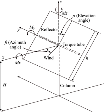
Fig. 1 Definition of relevant parameters of heliostat in coordinate system
The effect of the wind on heliostats is associated with natural characteristics of the wind, structural performance of the heliostat and the coupling interaction between both. In practical applications, the wind load coefficients are introduced, which can be expressed as
 ;
;
 ;
;
 ;
;
 ;
;
 ;
;
 (13)
(13)
where Fx, Fy and Fz stand for drag force, lateral force and lift force, respectively; Mx, My and Mz stand for lateral moment, pitching moment and azimuth moment at the hinge, respectively; CFx, CFy, CFz, CMx, CMy and CMz stand for the corresponding coefficients of the force and moment, respectively; A is the total area of the reflector; h is the height of the reflector plate;  is the mean wind speed at the height H (H is the height from the foundation to the center of the reflector and H=5 m).
Figure 2 shows the computational model of the heliostat in the numerical wind tunnel. The numerical wind tunnel is designed as 160 m length, 100 m width and 50 m height. The distance from the center of the heliostat to the velocity inlet is 40 m, and the maximum blocking rate of the model is 1.34%. The mean wind speed  20 m/s (fresh gale) which is applied in the velocity inlet and the wind speed profile with Davenport exponential law is used. A fully developed outflow boundary condition is employed. The top and side of the numerical wind tunnel are defined as free slip conditions; the heliostat and ground are defined as no slip conditions. In addition, the entire flow field is meshed by unstructured tetrahedral grids and structured hexahedral grids. And the total number of the grids is about 5.2��106. In order to describe the turbulent flow of the air near the ground, Reynolds averaged Navier-Stokes (RANS) equations which is based on time average method are employed and standard k-�� model is introduced to close turbulence equations [25].
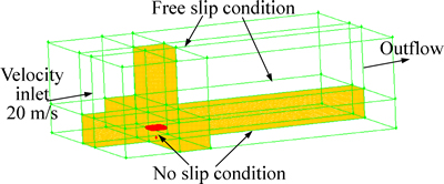
Fig 2 Computational model of heliostat in numerical wind tunnel (Grids in partial flow field region are hidden; The red color represents the heliostat, yellow represents the meshed grids and green represents the entire flow field)
3.2 Wind load coefficients analysis
The crucial for the safety of the heliostat under the strong wind is the accurate selection of the best stow position. PETERKA et al [5] suggested that the heliostat should be sent to a stow position that minimized wind drag on the reflector in the event of wind gusts condition. The heliostat has the smallest windward area when the heliostat is parallel to the wind direction, and therefore the elevation angle of 90�� for horizontal stow position and azimuth angle of 90�� for lateral stow position have been selected to evaluate the wind-resistant performance of the heliostat in various survival stow positions.
The mean wind load coefficients including the effect of the longitudinal and vertical wind loads in various survival stow positions are shown in Fig. 3. It is validated that the variation tendencies of the six curves by CFD simulation coincide well with the experimental results by PETERKA [5, 26]. Whether the elevation angle of 90�� or azimuth angle of 90��, the values of the drag coefficient CFx are all small and basically remain constant, and the main reason of which is the side of the reflector has the smallest windward area and roughly stays the same projected area in longitudinal wind speed direction. The lateral coefficient CFy is almost zero as the elevation angle ��=90�� because the flow around the reflector develops the very small wind pressure component along the y-axis. When the azimuth angle ��=90��, the space below the reflector increases with increasing ��, thus the wind pressure component along the y-axis decreases. As a result, the absolute values of the CFy decrease with increasing ��. The lift coefficient CFz has slight fluctuation and is always greater than zero which indicates the impact of the wind on the heliostat is upward.
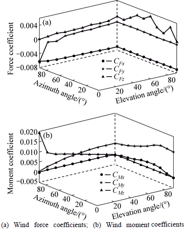
Fig. 3 Mean wind load coefficients in various survival stow positions:
The moments are caused by the non-uniform distribution of the wind loads on the reflector. Due to the amplification effect of the lever arm, the moment coefficients are large comparing with the force coefficients. The heliostat with sharp corners is regarded as a bluff body in the flow field. As the wind interacts with the heliostat, the incoming flow is separated at the windward edges of the reflector and then motions along the front and back surfaces of the reflector. The resultant force at the frontal part of the reflector shows the suction because the wind pressure on the back side is larger than that on the front side. The separated wind flow is rapid reattachment at the latter part of the reflector in which the resultant force presents the pressure. Due to the difference of the wind pressure distribution between the frontal and latter of the reflector, the pitching moment coefficient CMy is larger when ��=90��. Similarly, the azimuth moment coefficient CMz is larger when ��=90��. Moreover, the values of the lateral moment coefficient CMx are all small and almost keep constant.
In the stow position the heliostat is protected from the high storm wind speed, thus it is beneficial to improve the wind-resistant performance of the heliostat by minimizing wind load coefficients. Nevertheless, the differences of the wind load coefficients are unobvious in the different survival stow positions. Furthermore, the strength and stability of the heliostat are not only related to the wind load and its distribution but also associated with the structural stiffness. Only depending on the wind load coefficients is too hasty to determine the best survival stow position, and a further analysis for the wind-induced response of the heliostat is needed.
4 Results and discussion for stability analysis
4.1 Eigenvalue buckling analysis
Based on the discretization assumption the finite element model of the heliostat is established, as illustrated in Fig. 4. According to the structural feature of each component, the reflector, column and torque tube are defined as shell element, and the frame beam is defined as beam element.
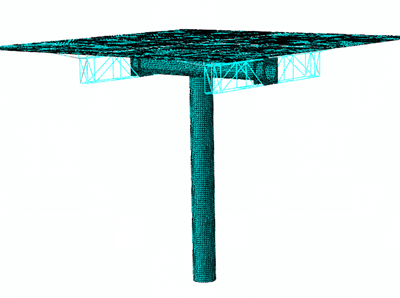
Fig. 4 Finite element model of heliostat
According to Eqs. (9)-(10), the first order eigenvalue buckling load coefficients of the heliostat are achieved by Lanczos method, as shown in Fig. 5. It can be seen that the ��1 is apparently different in the various survival stow positions. The ��1 reaches the maximum in the position of 90-90 and the minimum in the position of 00-90. An interest is that both have the identical azimuth angle and different elevation angle. According to the definition of the angles, the azimuth angle and elevation angle represent the wind direction and the state of the heliostat, respectively. Therefore, the safest and the least safe cases are only dependent on the state of the heliostat. Moreover, the ��1 approximately linearly increases with increasing �� when ��=90��, and the ��1 similarly exponentially increases with increasing �� when ��=90��.
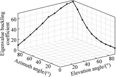
Fig. 5 First order eigenvalue buckling load coefficients in various survival stow positions
The variation trend indicates that the effect of the azimuth angle for the stability of the heliostat is greater than that of the elevation angle.
In reality the magnitude of the ��1 is correlated with the structural stiffness of the heliostat which includes linear elastic stiffness and initial stress stiffness. The linear elastic stiffness is determined by material properties. And the initial stress stiffness is determined by internal stress state and applied load. The wind pressure coefficients and their distributions on the reflector in the stow position of 00-90 and 90-90 are shown in Fig. 6 and Fig. 7, respectively. Due to the different elevation angle, the net wind pressure for each facet is completely different. The maximum for the structural stiffness of the heliostat is in the position of 90-90 and proportional to eigenvalue buckling load coefficient. As a result, the ��1 reaches the maximum in the position of 90-90.
In addition, the ��1 is always greater than 1 for all stow positions, which forecasts that buckling failure will not occur in the wind speed of 20 m/s condition.
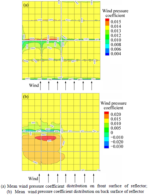
Fig. 6 Mean wind pressure coefficient distribution of reflector in stow position of 00-90:
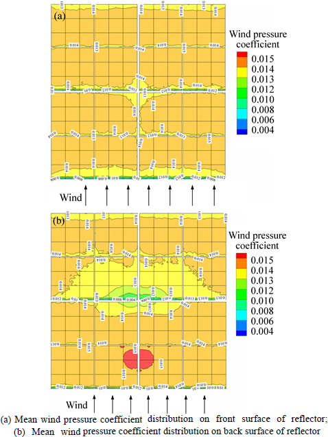
Fig. 7 Mean wind pressure coefficient distribution of reflector in stow position of 90-90:
However, the reference mean wind speed is only the nominal survival wind speed during the wind-resistant design of the heliostat. And the geometric nonlinearity, material nonlinearity and initial geometrical imperfection of the heliostat as well as longitudinal and vertical fluctuating wind are not taken into account. Therefore, the critical wind load is unreliable in accordance with eigenvalue buckling analysis for the ideal linear elastic structure. In order to guarantee the safety of the heliostat, the eigenvalue buckling load coefficient is larger and the wind-resistant stability is higher.
4.2 Nonlinear post-buckling analysis
The chief purpose of the structural stability is to evaluate the best survival stow position and maximal wind-resistant performance of the heliostat. If the eigenvalue buckling load coefficient in the minimal position is used as the design standard for wind-resistant performance, the safety of the heliostat in all stow positions can be warranted. Nonetheless, the stiffness characteristic of the braced structure and mechanical property of the material are not fully utilized, thereby the manufacturing cost of the heliostat increases to improve the wind-resistant safety factor. Hence, it is reasonable to select the stow position with the maximal eigenvalue buckling load coefficient. Furthermore, anemometers are installed to measure the wind speed and direction in the practical concentrating solar power field and the best survival stow position can be accurately located by controlling the drive unit of the heliostat. As a consequence, the survival stow position of 90-90 is selected to conduct the nonlinear post-buckling analysis and dynamic stability analysis in this and the following sections.
Above eigenvalue buckling analysis only predicts the theoretical critical wind load on heliostats, hence the nonlinear post-buckling behaviors of the heliostat in the full equilibrium process are investigated to obtain the true critical wind load. During the nonlinear post-buckling analysis, three significant influence factors are taken into account: the geometric nonlinearity caused by small strain and large deformation, the material nonlinearity caused by plastic deformation in local members and the initial geometrical imperfection caused by manufacturing deviation and installation error. Moreover, the bilinear kinematic hardening model [27] is used to express constitutive relation of steel, the equivalent von Mises stress is employed to distinguish material yield limit and the CIBAM is introduced to simulate the initial geometrical imperfection. The eigenvalue buckling load is taken as a given load in the nonlinear post-buckling analysis, and the post-buckling equilibrium process of the heliostat is investigated by Newton-Raphson method and arc length method [28]. The relevant material parameters are listed in Table 1.
Table 1 Material parameters for analysis
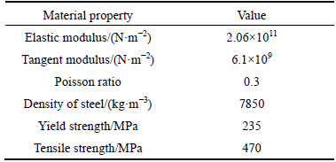
Table 2 lists the various calculation conditions for the heliostat. And the different load-displacement equilibrium curves of the heliostat in various cases are shown in Fig. 8. It can be observed that the post-buckling equilibrium curves of the cases 1-2 are significantly different from the cases 3-5. Since the geometric nonlinearity in cases 1-2 is not taken into account, the displacement of the heliostat linearly infinitely increases with increasing wind load. Consequently, an interest is that the heliostat has sustained bearing capacity and permanent stability, which means the instability for the heliostat will never occur. In these cases, the failure of the heliostat is mainly determined by the material properties and excessive deformation. In contrast, the post-buckling equilibrium curves are almost similar in cases 3-5. With increasing the wind load, the displacement of the heliostat increases and yet the structural stiffness decreases in the initial loading phase (Line AB). Because of the small nonlinear effect, the linear variation between the wind load and the displacement is presented. The heliostat is also in the stable equilibrium state. As the local components of the braced structure yield, the ever-increasing load induces the plastic zone extension of the material, thus the deformation of the heliostat accelerates (Line BC). In this phase, the structural stiffness weakens dramatically, while the equilibrium condition can be maintained by reducing the wind load on the reflector. Once the wind load exceeds the stable ultimate load (Point C), parts of the braced structure are failure due to local buckling, which induces the entire heliostat to lose the stability bearing capacity. The large sustained deformation is maintained under the small wind load, and the irrecoverable damage has already occurred. Furthermore, at the critical point of the post-buckling equilibrium curve, the wind load in cases 1-2 is 2.2 times that in cases 3-5 and far exceeds the critical load by the eigenvalue buckling analysis. Overall, the geometric nonlinearity which is based on the large deformation theory has a great effect on the stability bearing capacity for the heliostat, while the effects of the material nonlinearity and initial geometrical imperfection are relatively smaller. Therefore, during the wind-resistant stability design, the geometric nonlinearity should be preferentially considered and the material properties only need to meet the requirements.
Table 2 Various calculation conditions for heliostat
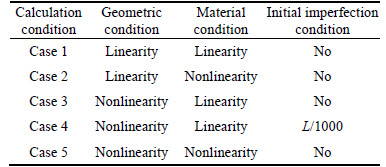
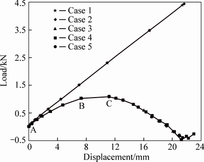
Fig. 8 Load-displacement equilibrium curves of heliostat in different cases
Figure 9 shows the influence of the different initial geometrical imperfections on the post-buckling behaviors of the heliostat. It can be deduced that the heliostat is insensitive to the initial geometrical imperfection, because the load-displacement equilibrium curves nearly remain consistent in the different initial imperfection conditions. The result is favorable to the manufacture, measurement and installation of the heliostat components. And the cost of the heliostat can be dramatically reduced because the high precision structural components are avoided. Moreover, it is also seen that the approximate linear relation between the wind load and the displacement of the heliostat is maintained in the initial loading phase. With increasing the wind load, the initial stress stiffness matrix of the heliostat increases thus the determinant of the tangent stiffness matrix decreases. The structural stiffness also decreases, and the slopes of the curves are gradually small. As the structural stiffness becomes singular, the stability bearing capacity of the heliostat reaches the limit. Once the wind load exceeds the stable ultimate load, the wind load declines linearly until the opposite equilibrium position. Simultaneously, the heliostat loses the stability bearing capacity rapidly due to nonlinear buckling. The different initial geometrical imperfections have an effect on opposite stable equilibrium position slightly. During the investigation, the maximum equivalent stress of the heliostat ��max=204 MPa which is less than the yield stress, and the critical load of the post- buckling behavior is 1082 N which is the eigenvalue buckling load of approximately 85%. That is, the heliostat will extremely survive as the actual mean wind speed is 7.5 times the designed survival wind speed. Hence, it indicates that the static stability of the heliostat is high in the stow position of 90-90.
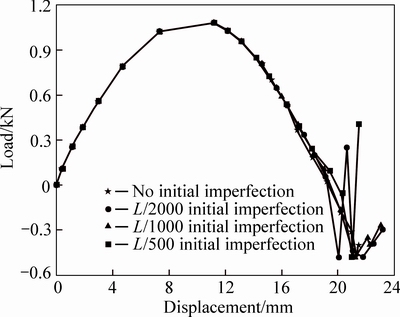
Fig. 9 Post-buckling behaviors of heliostat in different initial geometrical imperfections
4.3 Dynamic stability analysis
On account of introducing the time variable, the nonlinear dynamic stability of the heliostat is far more complicated than the static stability. Furthermore, dynamic buckling behavior has unique characteristics, such as dynamic critical load not only depends on structural style itself, but also relates to the duration of wind load and the dynamic properties of materials. And the dynamic buckling mode not only depends on the load distribution pattern, but also relates to the time-varying wind load. Nevertheless, the stochastic effect of the fluctuating wind is neglected in the process of the static stability analysis, which may make the heliostat unsafe. Thus, a comprehensive approach is proposed to evaluate the dynamic stability of the heliostat.
The power spectrum of the fluctuating wind pressure expresses the energy distribution of each frequency components in frequency domain. However, frequency domain analysis method which is based on the linear superposition principle can only investigate linear structure, thus time domain analysis method is introduced to research the strong nonlinear structure, such as the heliostat. The time domain analysis method can accurately provide correlation function of the structural response and transient behavior.
The top priority of the time domain analysis is to obtain the time history sample of the fluctuating wind load. The fluctuating wind consists of the longitudinal, vertical and transverse fluctuating components. Because of the weak cross correlation among the different directions, the correlative fluctuating components in the three-dimensional wind field can be simplified as the independent one-dimensional wind field in the three different directions [29]. In addition, the transverse fluctuating component has the negligible effect on the dynamic stability as the heliostat is in the stow position of 90-90. Consequently, only longitudinal and vertical fluctuating components are involved. The time history samples of the longitudinal and vertical fluctuating wind pressure are respectively shown in Fig. 10 and Fig. 11, which are derived by autoregressive model (AR model) [30]. The AR model has the advantages of small calculated amount and high simulation efficiency [31], thus it is widely used in the wind field simulation. The simulation time is 200 s. Comparison of the target power spectrums and the simulated power spectrums of the longitudinal and vertical fluctuating wind pressure are reasonably reliable because the natural characteristic of the atmospheric boundary layer wind is guaranteed and the spatial coherence is in good agreement.
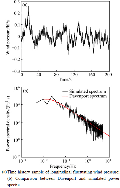
Fig. 10 Longitudinal fluctuating wind pressure simulation:(Double logarithmic coordinates)
As shown in Figs. 10 and 11, the stochastic process between the longitudinal and vertical fluctuating wind pressure is asynchronous. The vertical fluctuating wind pressure is overall less than the longitudinal. Nonetheless, the vertical peak wind pressure is nearly in the same order of magnitude compared with the longitudinal wind pressure. In addition, the longitudinal peak wind pressure is 0.26 kPa in 16.2 s, and the vertical peak wind pressure is 0.086 kPa in 66.8 s. Considering the maximal effect under the combined action of the longitudinal and vertical fluctuating wind pressure, the time history sample of the fluctuating wind pressure is selected from 10 s to 20 s for the dynamic stability analysis of the heliostat.
As the same as the static stability analysis, the geometric nonlinearity, material nonlinearity and initial geometrical imperfection are taken into account. The incremental dynamic analysis is used to increase the dynamic wind load gradually so that the maximum displacement response is derived at the various load amplitude coefficients. As shown in Fig. 12, the initial displacement is 2.7 mm due to the action of the gravity of the heliostat. The maximum displacement response of the heliostat nearly linearly increases with increasing �� when the load amplitude coefficient �ǡ�3.25, which indicates that the structural stiffness remains constant. Conversely, the maximum displacement response dramatically increases to 53 mm when ��=3.50. And the slope of the curve is very small in the process of 3.25 to 3.50, which signifies that the structural stiffness decreases sharply. A small increment induces the displacement response to increase significantly, thus ��=3.25 which can be taken as the critical wind load of the dynamic stability according to the B-R criterion. Actually, the tangent stiffness matrix of the heliostat has been non-positive definite when ��=3.5. The heliostat has not already borne the more load increment, so the dynamic responses of the displacement and stress are divergent. In this circumstance, the maximum equivalent stress ��max=527 MPa which is much more than the tensile strength. The heliostat is dynamic failure for losing the stability bearing capacity.
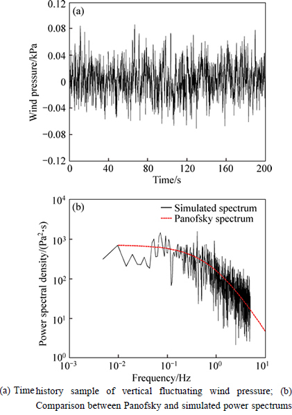
Fig. 11 Vertical fluctuating wind pressure simulation:(Double logarithmic coordinates)
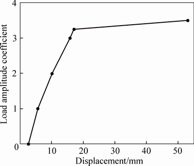
Fig. 12 Maximum displacement response of heliostat at various load amplitude coefficients
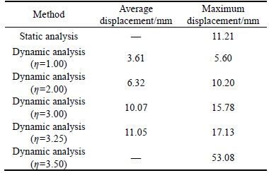
Figure 13 shows the time history curves of the maximum displacement and maximum equivalent stress at the various load amplitude coefficients. It can be observed that the variation trends of the curves are almost consistent for the different load amplitude coefficients. The envelope curve of the displacement response increases evenly with increasing �� when �ǡ�3.25. And the maximum equivalent stress is also less than the yield stress. The comparison between the static and dynamic displacement is listed in Table 3. It can be seen that the average displacement as ��=3.25 is close to the stable ultimate displacement by the static nonlinear post-buckling analysis, but the heliostat can still maintain stable vibration near the equilibrium position. Therefore, the heliostat is in the stable equilibrium state. Nevertheless, as the �� increases to 3.50, the displacement response increases significantly and the vibration of the heliostat diverges. In this case, partial components have been in the plastic stage. As the wind load reaches the peak value, the plastic zone has already developed rapidly which makes the structural stress exceed the tensile strength. The heliostat collapses for losing the stability bearing capacity. Furthermore, no evident weakening occurs for the structural stiffness, and no evident deviation from the equilibrium position of the vibration appears before the heliostat damages. Consequently, the sudden failure should be regarded as the dynamic instability of the heliostat. According to the equivalent displacement principle of the static and dynamic stability [32], the load amplitude coefficient ��=3.25 can be taken as the critical wind load of the dynamic stability. In other words, the heliostat will extremely survive in the stow position of 90-90 when the fluctuating wind speed is 36 m/s [33].
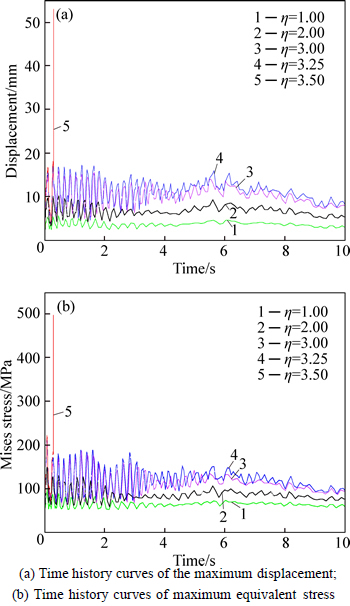
Fig. 13 Dynamic response curves of heliostat at various load amplitude coefficients:
Table 3 Comparison between static and dynamic displacement
5 Conclusions
1) The wind load coefficients are small in various survival stow positions and the differences are unobvious. Therefore, only depending on the wind load coefficients is too difficult to determine the best survival stow position for the heliostat.
2) Because of the coupling interaction between the wind field and structural stiffness, the eigenvalue buckling load coefficient of the heliostat reaches the maximum in the stow position of 90-90 which can be taken as the best survival stow position.
3) The geometric nonlinearity has a pronounced effect on the stability bearing capacity of the heliostat, while the effects of the material nonlinearity and initial geometrical imperfection are relatively small. Furthermore, the heliostat is insensitive to the initial geometrical imperfection, which is favorable to the manufacture, measurement and installation of the heliostat components.
4) The heliostat will extremely survive as the actual mean wind speed is 7.5 times the designed survival wind speed. Consequently, the heliostat has high stability bearing capacity and wind-resistant performance in the stow position of 90-90.
5) Combining the B-R criterion with equivalent displacement principle the dynamic critical wind speed and load amplitude coefficient are effectively evaluated. The results show the heliostat will extremely survive in the stow position of 90-90 as the fluctuating wind speed is 36 m/s.
References
[1] KOLB G J, JONES S A, DONNELLY M W, GORMAN D, THOMAS R, DAVENPORT R, LUMIA R. Heliostat cost reduction study [R]. New Mexico: Sandia National Laboratories, 2007.
[2] COVENTRY J, PYE J. Heliostat cost reduction-where to now? [C]// PITCHUMANI R. Energy Procedia. Amsterdam, Netherland: Elsevier Science BV, 2013: 60-70.
[3] YELLOWHAIR J, ANDRAKA C E. Evaluation of advanced heliostat reflective facets on cost and performance [C]// PITCHUMANI R. Energy Procedia. Amsterdam, Netherland: Elsevier Science BV, 2013: 265-274.
[4] SUN Hong-hang, GONG Bo, YAO Qiang. A review of wind loads on heliostat and trough collectors [J]. Renewable and Sustainable Energy Reviews, 2014, 32: 206-221.
[5] PETERKA J A, HOSOYA N, BIENKIEWICZ B, CERMAK J E. Wind load reduction for heliostats [R]. Colorado: Colorado State University, 1986.
[6] PETERKA J A, TAN Z, BIENKIEWICZ B, CERMAK J E. Mean and peak wind load reduction on heliostats [R]. Colorado: Colorado State University, 1987.
[7] PETERKA J A, TAN Z, BIENKIEWICZ B, CERMAK J E. Wind loads on heliostats and parabolic dish collectors [R]. Colorado: Colorado State University, 1988.
[8] PFAHL A, UHLEMANN H. Wind loads on heliostats and photovoltaic trackers at various Reynolds numbers [J]. Journal of Wind Engineering and Industrial Aerodynamics, 2011, 99: 964-968.
[9] PFAHL A, BUSELMEIER M, ZASCHKE M. Wind loads on heliostats and photovoltaic trackers of various aspect ratios [J]. Solar Energy, 2011, 85: 2185-2201.
[10] PFAHL A, BRUCKS A, HOLZE C. Wind load reduction for light-weight heliostats [C]// PITCHUMANI R. Energy Procedia. Amsterdam, Netherland: Elsevier Science BV, 2013: 193-200.
[11] GONG Bo, WANG Zhi-feng, LI Zheng-nong, ZANG Chun-cheng, WU Zhi-yong. Fluctuating wind pressure characteristics of heliostats [J]. Renewable Energy, 2013, 50: 307-316.
[12] GONG Bo, LI Zheng-nong, WANG Zhi-feng, WANG Ying-ge. Wind-induced dynamic response of heliostat [J]. Renewable Energy, 2012, 38: 206-213.
[13] ZANG Chun-cheng, GONG Bo, WANG Zhi-feng. Experimental and theoretical study of wind loads and mechanical performance analysis of heliostats [J]. Solar Energy, 2014, 105: 48-57.
[14] BLACKMON J B. Heliostat drive unit design considerations-site wind load effects on projected fatigue life and safety factor [J]. Solar Energy, 2014, 105: 170-180.
[15] DAVENPORT A G. The relationship of wind structures to wind loading [R]. Teddington, Middlesex: National Physical Laboratory, 1965: 54-102.
[16] ZHANG Xiang-ting. Calculation of structural wind pressure and wind vibration [M]. Shanghai: Tongji University Press, 1985. (in Chinese).
[17] GB50009-2012. Ministry of housing and urban-rural development of the PRC. load code for the design of building structures [S]. 2012. (in Chinese)
[18] European Convention for Constructional Steelwork, Technical Committee. T12: Wind effects recommendations for the calculation of wind effects on buildings and structures [S]. 1978.
[19] DEML M, WUNDERLICH W. Direct evaluation of the ��worst�� imperfection shape in shell buckling [J]. Computer Methods in Applied Mechanics and Engineering, 1997, 149: 201-222.
[20] CHEN Xin, SHEN Shi-zhao. Complete load-deflection response and initial imperfection analysis of single-layer lattice dome [J]. International Journal of Space Structures, 1993, 8(4): 271-278.
[21] American Institute of Steel Construction. ANSI/AISC, No. 360-05 Specification for Structural Steel Buildings [S]. 2005.
[22] ZHI Xu-dong, FAN Feng, SHEN Shi-zhao. Elasto-plastic instability of single-layer reticulated shells under dynamic actions [J]. Thin-Walled Structures, 2010, 48: 837-845.
[23] BUDIANSKY B, ROTH R S. Axisymmetric dynamic buckling of clamped shallow spherical shells [R]. Washington D C: NASA, 1962.
[24] VAMVATSIKOS D, CORNELL C A. Incremental dynamic analysis [J]. Earthquake Engineering & Structural Dynamic, 2002, 31(3): 491-514.
[25] VERSTEEG H K, MALALASEKERA W. An introduction to computational fluid dynamics: The finite volume method [M]. Second Edition. New Jersey: Prentice Hall, 2007.
[26] PETERKA J A, DERICKSON R G. Wind load design methods for ground-based heliostats and parabolic dish collectors [R]. Colorado: Colorado State University, 1992.
[27] RAHMAN S M, HASSAN T, CORONA E. Evaluation of cyclic plasticity models in ratcheting simulation of straight pipes under cyclic bending and steady internal pressure [J]. International Journal of Plasticity, 2008, 24(10): 1756-1791.
[28] FORDE W R B, STIEMER S F. Improved arc length orthogonality methods for nonlinear finite element analysis [J]. Computers and Structures, 1987, 27(5): 625-630.
[29] LI Jin-hua, LI Chun-xiang. Development of numerical simulations for stochastic wind fields in civil engineering [J]. Journal of Vibration and Shock, 2008, 27(9): 116-125. (in Chinese).
[30] OWEN J S, ECCLES B J, CHOO B S, WOODINGS M A. The application of auto-regressive time series modelling for the time- frequency analysis of civil engineering structures [J]. Engineering Structures, 2001, 23: 521-536.
[31] IANNUZZI A, SPINELLI P. Artificial wind generation and structural response [J]. Journal of Structure Engineering, 1987, 113(12): 2382-2398.
[32] LI Yuan-qi, TAMURA Y. Nonlinear dynamic analysis for large-span single-layer reticulated shells subjected to wind loading [J]. Wind and Structures, 2005, 8(1): 35-48.
[33] CUTTING F M. Heliostat survivability and structural stability for wind loading [C]// Alternative Energy Sources. Washington D C: Hemisphere Publishing Corp, 1978: 463-525.
(Edited by YANG Hua)
Foundation item: Project(CYB14010) supported by Chongqing Graduate Student Research Innovation Project, China; Project(51405209) supported by the National Natural Science Foundation of China
Received date: 2015-07-02; Accepted date: 2015-12-14
Corresponding author: CHEN Xiao-an, Professor, PhD; Tel: +86-23-65106006; E-mail: xachen@cqu.edu.cn
Abstract: Heliostats are sensitive to the wind load, thus as a key indicator, the study on the static and dynamic stability bearing capacity for heliostats is very important. In this work, a numerical wind tunnel was established to calculate the wind load coefficients in various survival stow positions. In order to explore the best survival stow position for the heliostat under the strong wind, eigenvalue buckling analysis method was introduced to predict the critical wind load theoretically. Considering the impact of the nonlinearity and initial geometrical imperfection, the nonlinear post-buckling behaviors of the heliostat were investigated by load-displacement curves in the full equilibrium process. Eventually, combining B-R criterion with equivalent displacement principle the dynamic critical wind speed and load amplitude coefficient were evaluated. The results show that the determination for the best survival stow position is too hasty just by the wind load coefficients. The geometric nonlinearity has a great effect on the stability bearing capacity of the heliostat, while the effects of the material nonlinearity and initial geometrical imperfection are relatively small. And the heliostat is insensitive to the initial geometrical imperfection. In addition, the heliostat has the highest safety factor for wind-resistant performance in the stow position of 90-90 which can be taken as the best survival stow position. In this case, the extreme survival wind speeds for the static and dynamic stability are 150 m/s and 36 m/s, respectively.
