
J. Cent. South Univ. (2017) 24: 2961-2968
DOI: https://doi.org/10.1007/s11771-017-3710-7

Regularized inversion for coseismic slip distribution with active constraint balancing
TONG Xiao-zhong(ͯТ��)1, 2, XIE Wei(лά)1, GAO Da-wei(�ߴ�ά)2
1. School of Geosciences and Info-physics, Central South University, Changsha 410083, China;
2. School of Earth and Ocean Sciences, University of Victoria, Victoria, British Columbia V8P 5C2, Canada
 Central South University Press and Springer-Verlag GmbH Germany, part of Springer Nature 2017
Abstract:
Estimating the spatial distribution of coseismic slip is an ill-posed inverse problem, and solutions may be extremely oscillatory due to measurement errors without any constraints on the coseismic slip distribution. In order to obtain stable solution for coseismic slip inversion, regularization method with smoothness-constrained was imposed. Trade-off parameter in regularized inversion, which balances the minimization of the data misfit and model roughness, should be a critical procedure to achieve both resolution and stability. Then, the active constraint balancing approach is adopted, in which the trade-off parameter is regarded as a spatial variable at each model parameter and automatically determined via the model resolution matrix and the spread function. Numerical experiments for a synthetical model indicate that regularized inversion using active constraint balancing approach can provides stable inversion results and have low sensitivity to the knowledge of the exact character of the Gaussian noise. Regularized inversion combined with active constraint balancing approach is conducted on the 2005 Nias earthquake. The released moment based on the estimated coseismic slip distribution is 9.91��1021 N��m, which is equivalent to a moment magnitude of 8.6 and almost identical to the value determined by USGS. The inversion results for synthetic coseismic uniform-slip model and the 2005 earthquake show that smoothness-constrained regularized inversion method combined with active constraint balancing approach is effective, and can be reasonable to reconstruct coseismic slip distribution on fault.
Key words:
1 Introduction
The inverse problem for coseismic slip distribution is usually underdetermined and ill-posed, meaning that small errors in the observed data can lead to huge changes in the model. In order to stabilize the inversion and to produce useful solutions, regularization constraints are imposed on the model. A typical regularization scheme is to minimize the norm or a semi-norm of the model, such as smoothing or damping [1�C4]. To get both high resolution and stable inversion, great care must be taken in balancing the minimization of the data fitting error and the amount of regularization.
A trade-off (or regularization) parameter is introduced to balance between the data misfit and the model norm and is usually a single number that is globally applied to the entire model. Different strategies are used to determine the optimum trade-off parameter when the observations are contaminated with Gaussian noise of uniform, but unknown, standard deviation. BARNHART and LOHMAN [5] choose the trade-off parameter using the jRi method, an approach that balances the contribution from data noise (perturbation error) and over-smoothing (regularization error). XU et al [6] proposed a coseismic slip distribution inversion method based on variance component estimation, which not only determines the weight of different data sets but also can get the smoothing factor value. YABUKI and MATSU��URA [7] choose the value that minimizes the Akaike Bayesian information criterion (ABIC). Other popular techniques for choosing the trade-off parameter include identifying the corner of the L-curve criterion [8, 9], and the generalized cross-validation (GCV) criterion [10]. Nevertheless, these methods cannot quantitatively or automatically optimize the model resolution and the stability.
In this work, the smoothness-constrained least- squares inversion method combined with active constraint balancing approach is adopted for reconstructing coseismic slip distribution. Firstly, the model resolution matrix and the spread function in the smoothness-constrained least-squares inversion for Gaussian noise data are proposed, through which the active constraint balancing approach for trade-off parameter can be determined. Secondly, a synthetic strike-slip coseismic model is used to verify the efficiency of the active constraint balancing technique scheme. In order to check the stableness of the algorithm, numerical experiments for Gaussian distribution noise data are carried out. Finally, a field example of the 2005 Nias earthquake is shown for demonstrating the reconstruction of coseismic slip distribution using the active constraint balancing technique.
2 Inversion methodology
2.1 Smoothness-constrained least-squares inversion
The inverse problem to be solved for distributed coseismic slip can be written as follows:
Gm=d (1)
where G is a matrix of Green��s functions which relate coseismic slip on a dislocation at depth to displacements at a free surface; d is a data vector of dimension p consisting of single-component surface deformation; m is a parameter vector of dimension 2M consisting of M slip vectors each having two degrees of freedom. If the data are two- or three-component displacements of N GPS stations, then p=2N or 3N, respectively, but the data can also be a mixture of displacements, strains, and tills. The two directions of freedom for each slip vector can be its two components in the local strike and dip directions of the fault element but can also be a vector norm and a directional measure or other derived parameters. To derive Green��s functions, field equations that assume either a rectangular or triangular slipping dislocation within an isotropic elastic half-space can be used [11, 12].
When solving inverse problems, it needs to seek a solution that predicts the observed data to a certain degree consistent with data noise and, at the same time, satisfies certain constraints, such as the smoothness in a given direction. To achieve both, a total objective function to be minimized is often constructed. A generic form usually consists of two terms: data misfit and model objective function. The first part is used to quantify how well the observed data are reproduced by the inverse solution, and we impose constraints on the complexity and smoothness of the recovered model in the second term. These two terms are combined by using a trade-off parameter �� [13]:
 (2)
(2)
where fd is the data misfit term, fm is the model structure term and �� is known as trade-off parameter (regularization parameter), that balances between fd and fm.
For inversions that use L2 norm to measure the size of vectors, the objective function is given by
 (3)
(3)
where dobs is the observed data, D=[Dss 0; 0 Dds] is a Laplacian operator, including the two smoothness matrixes Dss and Dds for the strike-slip and dip-slip, Wd is a diagonal data weighting matrix whose elements are reciprocals of the standard deviations of noise in observed data,  where ��i is the standard deviation of the noise in the ith datum.
In order to solve the linear minimization problem Eq.(3), a weighted damped smoothness-constrained least-squares approach can be used as follows:
 (4)
(4)
The finite difference approximation for m recast into a two-dimensional array, s, having column and row indices i and j, implements Laplace��s equation [14]:
 (5)
(5)
where ��x and ��y are the respective the along-strike and surface projection of the down-dip fault patch dimensions. For example, the smoothness matrix for strike-slip Dss can be constructed as follows:
 (6)
(6)
Here nc represents the number of the down-dip fault patches.
2.2 Determination of trade-off parameter
Determination of the trade-off parameter, which balances the minimization of the data misfit and model roughness, may be a critical procedure to achieve both resolution and stability. A large trade-off parameter, in principle, would apply more constraint or regularization to the solution and give poor resolution of the model parameters. On the other hand, too small trade-off parameter may be harmful to the stability of the inversion. In our implementation, the active constraint balancing scheme is adopted, in which the trade-off parameter is regarded as a spatial variable at each model parameter and automatically determined via the model resolution matrix and the spread function [15].
The active constraint balancing algorithm has been implemented to obtain an optimal smoothness constraint. According to this algorithm, the trade-off parameter can be set optimally by the spread function SPi of the ith model parameter, which is defined by the model resolution matrix R [16, 17]. Combined with the diagonal data weighting matrix, the model resolution matrix can be expressed as
 (7)
(7)
where
 (8)
(8)
The model resolution matrix illustrates how well resolved each model parameter is given the data kernel and a priori model inputs [17]. In cases where m is uniquely determined, R is an identity matrix. Otherwise, R reflects the relationship between the inverted model as a spatial averaging of the true model, such that:
 (9)
(9)
The spread function, which accounts for the inherent degree of how much the ith model parameter is not resolvable, is defined as [18]
 (10)
(10)
where M is the total number of inversion parameters, ��ij is a weighting factor defined by the spatial distance between the ith and jth model parameters, and Sij is a factor which accounts for whether the constraint or regularization is imposed on the ith parameter and its neighboring parameters. The value of Sij is unity when Dij in Eq. (4) is nonzero, and it is zero when Dij equals zero. In other words, the spread function defined here is the sum of the squared spatially weighted spread of the ith model parameter with respect to all model parameters excluding ones upon which a smoothness constraint is imposed. In this approach, the trade-off parameter �� is set by a value from log-linear interpolation.
According to the spread functions, trade-off parameters are set linearly in logarithmic space between preselected lower and upper limit values. Logarithmic space is used because the spread function varies in an exponential manner with the location of model parameters, and goodness of resolution is expected to inversely proportional to the logarithm of the spread function. The following formula assigns the trade-off parameter according to the spread function [19]:
 (11)
(11)
where ��i is the trade-off parameter for the model parameter i;  is the spread function for the model parameter i;
  and
and  are the minimum and maximum values of spread function, respectively; ��min and ��max are the minimum and maximum values of the trade-off parameter, which must be provided in advance.
Through extensive numerical experiments, ��min and ��max can be obtained when the trade-off parameters are selected as the minimum and the maximum row sum of the matrix product  Therefore, the ��min and ��max can be given as follows:
 (12)
(12)
and
 (13)
(13)
where amj is an indicated element of  and M is the number of model parameters.
3 Synthetic tests
3.1 Inversion of synthetic model
A synthetic strike-slip coseismic model shown in Fig. 1(a) is used to verify the efficiency of the active constraint balancing technique. A rupture area is selected on this fault with a length of 12 km and width of 8 km, consisting of 24��16=384 sub-faults, each 20 km�� 20 km in size. The top of the fault is at a depth of 2 km, with a fault plane of strike=0��, dip=90�� and rake=0��. The synthetic strike-slip model is assumed of uniform coseismic slip distribution, and its value is 10 m.
The inverted model using active constraint balancing approach with ��min=0.0006 and ��max=0.0061 is in Fig. 1(b), which can effectively recover the coseismic slip distribution. The distribution of spread functions and trade-off parameters is shown in Figs. 1(c) and (d), respectively. Based on the distribution of spread functions, the optimized spatially varying trade-off parameters are assigned to the model parameters with values between 0.0006�C0.0061 and the calculated distribution of the trade-off parameters shows a trend similar to that of the spread functions. Thus, for highly resolvable model parameters, a small value of the trade-off parameter is assigned and vice versa. The optimized constraint can enhance the stability of the inversion process and aids in maintaining the model resolution.
Moreover, a comparison between observed and predicted coseismic displacements, as shown in Fig. 2,shows very good agreement in three-component surface deformation. In Fig. 2, the white arrows represent horizontal coseismic displacements and the contour map represents vertical coseismic displacements. The released moment based on the estimated coseismic slip distribution is 2.59��1021 N��m (using a value of 40 GPa for rigidity), which agrees well with 2.48��1021 N��m from the synthetic model. The moment magnitude calculated from coseismic slip distribution is Mw=8.2 and almost identical to the value determined by the synthetic model. Therefore, the inversion result for synthetic coseismic uniform-slip model shows that smoothness-constrained regularized inversion method combined with active constraint balancing approach is effective, and can be reasonable to reconstruct coseismic slip distribution on fault.
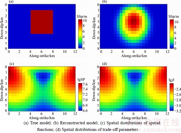
Fig. 1 Trade-off solution for a coseismic slip model:
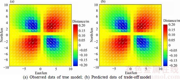
Fig. 2 Coseismic displacement of synthetic model and inversion results:
3.2 Inversion of noise data
To test the stableness of the inverse algorithm, numerical experiments for coseismic noise data are implemented, through which the Gaussian noises are added to the synthetic data. In probability theory, the Gaussian (or normal) distribution is a very common continuous probability distribution. Gaussian distributions are important in statistics and are often used in the natural and social sciences to represent real-valued random variables whose distributions are not known [20]. The Gaussian distribution describes a special class distribution that is symmetric and can be described as N(��, ��) by the mean �� and the standard deviation �� of the distribution [21].
The results of the inversion for noise levels of N(0.0.01), N(0.0.05), N(0.0.10) and N(0.0.20), corresponding to the coseismic displacements from the synthetic model in Fig. 2(a), are shown in Fig. 3. All the inverted models can effectively reconstruct the coseismic slip distribution, and no manifestation of artificial structure caused by fitting the noise is observed. However, with the increasing of noise level, there will be a more detailed difference between inverted model and synthetic model.
For the different noise level of N(0.0.01), N(0.0.05), N(0.0.10) and N(0.0.20), the optimized spatially varying trade-off parameters are assigned to the model parameters with values between 6.0094�C60.7990, 0.2408�C2.4320, 0.0602�C0.6080 and 0.0150�C0.1520, respectively. The trade-off parameters determined by active constraint balancing approach show a trend similar to that of the spread functions and have low sensitivity to the knowledge of the exact character of the noise. Therefore, the inversion results for Gaussian noise data show that smoothness-constrained regularized inversion method approach is stable and the active constraint balancing approach can be worked well in estimating the trade-off parameters.
4 Application to 2005 Nias earthquake
4.1 Observation data
The Mw 8.7 Nias earthquake of 28 March 2005 happened three months after the Mw 9.2 December 26, 2004, Aceh-Andaman earthquake and may be the largest aftershock ever recorded. It was recorded by a network of nearby continuous GPS stations, namely the Sumatra GPS Array (SuGAr). There are 10 GPS stations, including nine SuGAr and the station SAMP, installed by the Indonesian National Surveying Agency. Three sites (LEWK, BSIM, and LHWA) were installed about a month before the Nias earthquake; three sites (PBAI, PSMK, and PTLO) just south of the Equator were installed in mid-2002; and another three sites were installed in the few months between the Aceh-Andaman and Nias earthquakes [22].
The estimated geodetic coseismic offsets for the Nias earthquake are listed in Table 1. From Table 1, it can be clearly observed that the maximum value of horizontal coseismic displacements and the maximum value of vertical coseismic displacements are about 4.5 m and 2.9 m, respectively.
4.2 Inversion results
A rupture area for regularized inversion is selected on this fault with a length of 400 km and width of 340 km, consisting of 20��34=680 sub-faults, each 20 km��10 km in size. The top of the fault is at a depth of 3 km, with a fault plane of strike=325�� and dip=10��.
The inverted model using active constraint balancing approach with ��min=12.0236 and ��max=9.5433�� 104 is shown in Fig. 4. The observed and predicted horizontal coseismic displacements, as shown in Fig. 4 with blue arrows and red arrows, show very good agreement in two-component surface deformation. Figures 4(a) and (b) show the strike-slip distribution and the dip-slip distribution with the maximum value 3.6 m and 12.6 m.
The inversion result of total-slip distribution shown in Fig. 4(c) with the maximum value 12.8 m, which agrees well spatially with the coseismic slip distribution generated by KONCA et al [23] and HSU et al [24]. The released moment based on the estimated coseismic slip distribution is 9.91��1021 N��m (using a value of 40 GPa for rigidity), which agrees well with 1.00��1022 N��m from KONCA et al [23]. The moment magnitude calculated from coseismic slip distribution is Mw=8.6 and almost identical to the value determined by USGS.
5 Conclusions
1) An algorithm of smoothness-constrained regularized inversion combined with the active constraint balancing scheme is presented. The algorithm is effective and can be reasonable to reconstruct uniform and non- uniform coseismic slip distribution on fault.
2) Numerical experiments showed that the active constraint balancing approach, which uses spatially varying trade-off parameters, can provides stable inversion results. The active constraint balancing approach for choosing the trade-off parameters has the advantages of not requiring manual choice of a ��corner�� as L_curve method mentioned, and having low sensitivity to the knowledge of the exact character of the noise.
3) The algorithm is employed to inverse the non- uniform slip distribution of the 2005 Nias earthquake from GPS data. The trade-off solution shows that the maximum total-slip is 12.8 m, which agrees well spatially with the coseismic slip distribution generated by other researchers. The total seismic moment is about 9.91��1021 N��m, which corresponds to Mw=8.6 and almost identical to the value determined by USGS.
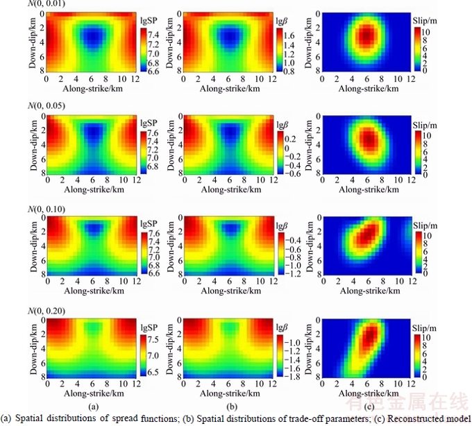
Fig. 3 Numerical experiments with regularized inversion for Gaussian distribution noise data:
Table 1 Coseismic displacement of GPS sites for March 28, 2005, Nias earthquake
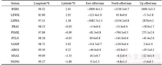
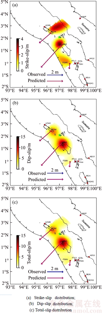
Fig. 4 Inversion results of coseismic slip distribution for 2005 Nias earthquake:
References
[1] MASTERLARK T. Finite element model predictions of static deformation from dislocation source in a subduction zone: Sensitivities to homogeneous, isotropic, Poisson-solid, and half-space [J]. Journal of Geophysical Research, 2003, 108(B11): 2540�C2556.
[2] MAERTEN F, RESOR P, POLLARD D, MAERTEN L. 2005. Inverting for slip on three-dimensional fault surfaces using angular dislocations [J]. Bulletin of the Seismological Society of America, 2005, 95(5): 1654�C1665.
[3] WANG Yong-zhe, ZHU Jia-jun, OU Zi-qiang, LI Zhi-wei, XING Xue-min. Coseismic slip distribution of 2009 L��Aquila earthquake derived from InSAR and GPS data [J]. Journal of Central South University, 2012, 19(1): 244�C251.
[4] FARQUHARSON C G, OLDENBURG D W. A comparison of automatic techniques for estimating the regularization parameter in non-linear inverse problems [J]. Geophysical Journal International, 2004, 156(3): 411�C425.
[5] BARNHART W D, LOHMAN R B. Automated fault model discretization for inversions for coseismic slip distributions [J]. Journal of Geophysical Research, 2010, 115(10): B10419.
[6] XU C J, DENG C Y, ZHOU L X. Coseismic slip distribution inversion method based on the variance component estimation [J]. Geomatics and Information Science of Wuhan University, 2016, 41(1): 37�C44. (in Chinese)
[7] YABUKI T, MATSU��URA M. Geodetic data inversion using a Bayesian information criterion for spatial distribution of fault slip [J]. Geophysical Journal International, 1992, 109(2): 363�C375.
[8] JIANG G Y, XU C J, WEN Y M. Inversion for coseismic slip distribution of the 2010 Mw6.9 Yushu Earthquake from InSAR data using angular dislocations [J]. Geophysical Journal International, 2013, 181(3): 1441�C1458.
[9] HREINSD TTIR S, FREYMUELLER J T, FLETCHER H J, LARSEN C F. Coseismic slip distribution of the 2002 Mw7.9 Denali fault earthquake, Alaska, determined from GPS measurements [J]. Geophysical Research Letters, 2003, 30(13): 1670.
[10] CHEN Shao-hua, ZHU Zi-qiang, LU Guang-yin, CAO Shu-jin. Inversion of gravity gradient tensor based on preconditioned conjugate gradient [J]. Journal of Central South University: Science and Technology, 2013, 44(2): 619�C625. (in Chinese)
[11] OKADA Y. Surface deformation due to shear and ensile faults in a half-space [J]. Bulletin of the Seismological Society of America, 1985, 75(4): 1135�C1154.
[12] OKADA Y. Internal deformation due to shear and ensile faults in a half-space [J]. Bulletin of the Seismological Society of America, 1992, 82(2): 1018�C1040.
[13] SUN J J, LI Y G. Adaptive Lp inversion for simultaneous recovery of both blocky and smooth features in a geophysical model [J]. Geophysical Journal International, 2014, 197(2): 882�C899.
[14] TONG Xiao-zhong, LIU Jian-xin, GUO Rong-wen, LIU Hai-fei. Three-dimensional magnetotelluric regularized inversion based on smoothness-constrained model [J]. Transactions of Nonferrous Metals Society of China, 2014, 24(2): 509�C513.
[15] YI M J, KIM J H, CHUNG S H. Enhancing the resolving power of least-squares inversion with active constraint balancing [J]. Geophysics, 2003, 68(3): 931�C941.
[16] MENKE W. Geophysical data analysis: discrete inverse theory [M]. New York: Academic Press, Inc., 2012.
[17] AN M. A simple method for determining the spatial resolution of a general inverse problem [J]. Geophysical Journal International, 2012, 191(2): 849�C864.
[18] JOO Y, SEOL S J, BYUN J. Acoustic full-waveform inversion of surface seismic data using the Gauss-Newton method with active constraint balancing [J]. Geophysical Prospecting, 2013, 61(S1): 166�C182.
[19] LEE S K, KIM H J, SONG Y, LEE C K. MT2DinvMatlab-A program in MATLAB and FORTRAN for two-dimensional magnetotelluric inversion [J]. Computers and Geosciences, 2009, 35(8): 1722�C1734.
[20] CHAVE A D, LEZAETA P. The statistical distribution of magnetotelluric apparent resistivity and phase [J]. Geophysical Journal International, 2007, 17(1): 127�C132.
[21] LI Dun-zhu, HUANG Qing-hua, CHEN Xiao-bin. Error effects on magnetotelluric inversion [J]. Chinese Journal of Geophysics, 2009, 52(1): 268�C274. (in Chinese)
[22] KREEMER C, BLEWITT G, MAERTEN F. Co- and postseismic deformation of the 28 March 2005 Nias Mw8.7 earthquake from continuous GPS data [J]. Geophysical Research Letters, 2006, 33(7): L07307.
[23] KONCA A O, HIORLEIFSDOTTIR V, SONG T A. Rupture kinematics of the 2005, Mw 8.6, Nias-Simeulue earthquake from the joint inversion of seismic and geodetic data [J]. Bulletin of the Seismological Society of America, 2007, 97(1): 307�C322.
[24] HSU Y J, SIMONS M, WILLIAMS C, CASAROTTI E. Three- dimensional FEM derived elastic Greens��s functions for the coseismic deformation of the 2005 Mw8.7 Nias-Simeulue, Sumatra earthquake [J]. Geochemistry Geophysics Geosystems, 2011, 12(7): Q07013.
(Edited by HE Yun-bin)
Cite this article as:
TONG Xiao-zhong, XIE Wei, GAO Da-wei. Regularized inversion for coseismic slip distribution with active constraint balancing [J]. Journal of Central South University, 2017, 24(12): 2961.
DOI:https://dx.doi.org/https://doi.org/10.1007/s11771-017-3710-7Foundation item: Projects(41604111, 41541036) supported by the National Natural Science Foundation of China
Received date: 2016-12-29; Accepted date: 2017-04-08
Corresponding author: XIE Wei, Associate Professor, PhD; Tel: +86�C13574881853; E-mail: xw76676372@126.com
Abstract: Estimating the spatial distribution of coseismic slip is an ill-posed inverse problem, and solutions may be extremely oscillatory due to measurement errors without any constraints on the coseismic slip distribution. In order to obtain stable solution for coseismic slip inversion, regularization method with smoothness-constrained was imposed. Trade-off parameter in regularized inversion, which balances the minimization of the data misfit and model roughness, should be a critical procedure to achieve both resolution and stability. Then, the active constraint balancing approach is adopted, in which the trade-off parameter is regarded as a spatial variable at each model parameter and automatically determined via the model resolution matrix and the spread function. Numerical experiments for a synthetical model indicate that regularized inversion using active constraint balancing approach can provides stable inversion results and have low sensitivity to the knowledge of the exact character of the Gaussian noise. Regularized inversion combined with active constraint balancing approach is conducted on the 2005 Nias earthquake. The released moment based on the estimated coseismic slip distribution is 9.91��1021 N��m, which is equivalent to a moment magnitude of 8.6 and almost identical to the value determined by USGS. The inversion results for synthetic coseismic uniform-slip model and the 2005 earthquake show that smoothness-constrained regularized inversion method combined with active constraint balancing approach is effective, and can be reasonable to reconstruct coseismic slip distribution on fault.
