
J. Cent. South Univ. (2012) 19: 1425-1436
DOI: 10.1007/s11771-012-1159-2![]()
Performance-based seismic financial risk assessment of reinforced concrete frame structures
Wu Qiao-yun(������)1,2, Zhu Hong-ping(���ƽ)1,2, FAN Jian(����)1,2
1. School of Civil Engineering and Mechanics, Huazhong University of Science and Technology, Wuhan 430074, China;
2. Hubei Key Laboratory of Control Structures, Huazhong University of Science and Technology,Wuhan 430074, China
? Central South University Press and Springer-Verlag Berlin Heidelberg 2012
Abstract:
Engineering facilities subjected to natural hazards (such as winds and earthquakes) will result in risk when any designed system (i.e. capacity) will not be able to meet the performance required (i.e. demand). Risk might be expressed either as a likelihood of damage or potential financial loss. Engineers tend to make use of the former (i.e. damage). Nevertheless, other non-technical stakeholders cannot get useful information from damage. However, if financial risk is expressed on the basis of probable monetary loss, it will be easily understood by all. Therefore, it is necessary to develop methodologies which communicate the system capacity and demand to financial risk. Incremental dynamic analysis (IDA) was applied in a performance-based earthquake engineering context to do hazard analysis, structural analysis, damage analysis and loss analysis of a reinforced concrete (RC) frame structure. And the financial implications of risk were expressed by expected annual loss (EAL). The quantitative risk analysis proposed is applicable to any engineering facilities and any natural hazards. It is shown that the results from the IDA can be used to assess the overall financial risk exposure to earthquake hazard for a given constructed facility. The computational IDA-EAL method will enable engineers to take into account the long-term financial implications in addition to the construction cost. Consequently, it will help stakeholders make decisions.
Key words:
1 Introduction
Recently, the Pacific Earthquake Engineering Research (PEER) Center has developed a new evaluation methodology for performance-based earthquake engineering (PBEE) [1-2], which is based on the triple integral total probability equation. Such an equation is useful for engineers and designers, but gives little information to those non-technical stakeholders (such as owners, insurers, policy makers and investors) to make better decisions and strategies. Therefore, it needs to develop the concepts of the seismic-specific methodology and extend it to an all hazards framework so that all stakeholders can easily get available information from it.
The proposed PBEE gets the widespread acceptance [2-7] since the introduction and it is considered to be a sound basis for further development. The implementation of PBEE in quantitative evaluation of the performance of a given building (either an existing building or a completed design of a new building) is denoted as performance-based assessment (PBA) [8-9]. PBA can provide stakeholders with information about the building (usually expressed in probabilistic terms) that facilitates informed decision making for risk management, and risk will be easily understood by all stakeholders if expressed in monetary terms rather than in terms of technical parameters representing performance measures.
In this work, the PEER triple integral formulation is augmented to give an additional dimension and time. By aggregating losses over time and expressing it in monetary terms, useful information can be made available to the non-technical stakeholders. The incremental dynamic analysis (IDA) process is developed specifically for reinforced concrete (RC) frame structures. The IDA results are quantitatively modeled and then integrated into a probabilistic risk analysis procedure, which takes into account all the uncertainties (aleatory and epistemic uncertainties) involved. Confidence intervals and damage outcomes for given hazard intensity levels, such as the design basis earthquake (DBE) or a maximum considered earthquake (MCE), can be evaluated. Then, the proposed methodology can be applied to estimating the financial risk of a RC frame structure due to seismic hazards.
2 Performance-based assessment
The performance based assessment (PBA) methodology developed in PEER Center [8-9] involves four types of random variables and incorporates four consecutive stages which are shown in Fig. 1. The four variables are denoted as: intensity measure (IM), engineering demand parameter (EDP), damage measure (DM) and decision variable (DV). The IM (I) describes the intensity of a ground motion (e.g. spectral acceleration associated with 5% damping at the first mode period of the building, Sa(T1, 5%)); the EDP (E) is a structural response parameter (e.g. maximum interstorey drift, ��max); the DM (DM) quantifies the level of damage to a building component; the DV (DV) describes the performance of building (e.g. monetary loss).
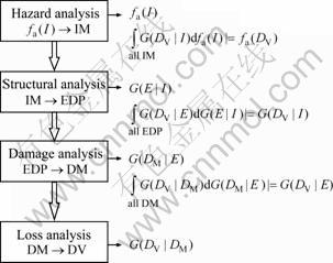
Fig. 1 Performance-based assessment methodology layout
2.1 Hazard analysis
In hazard analysis, the probability of an earthquake of a region within certain period is studied. The main outcome of hazard analysis is a seismic hazard curve which shows the relationship between an IM and its annual frequency of exceedance (i.e. fa(I)). Herein, the IM could be a scalar or a vector. Traditionally, Sa(T1, 5%) (i.e. scalar IM) has been used as the IM for its simplicity and easiness of computational work. Recently, the use of variable IM has shown some advantages in describing ground motion characteristics [6, 10-11], especially in the case of near fault ground motions [12-14].
In hazard analysis, it is necessary to define the relationship between IM and its annual frequency fa, which is commonly known as the hazard�Crecurrence relationship. By fitting a straight line through two known points in a log�Clog scale, it is possible to approximate the hazard�Crecurrence curve by the following equation [1]:
![]() (1)
(1)
where k and k0 are empirical constants, and they can be determined by the following equations:
![]() (2)
(2)
![]()
![]() (3)
(3)
where![]() and
and![]() are the annual exceeding probabilities represented by 10% and 2% in 50-year ground motions, respectively;
are the annual exceeding probabilities represented by 10% and 2% in 50-year ground motions, respectively;![]() and
and![]() are the spectral accelerations represented by 10% and 2% in 50-year ground motions (i.e. DBE and MCE), respectively.
are the spectral accelerations represented by 10% and 2% in 50-year ground motions (i.e. DBE and MCE), respectively.
2.2 Structural analysis
Given the information provided by seismic hazard analysis, the representative ground motions and an analytical model of the engineered facility, a variable of structural response parameters (E) is obtained in the structural analysis stage. The relationship between I and E can be obtained through multi-intensity inelastic response analyses of the analytical model which incorporates the structural system, non structural system, and geotechnical aspects of the structure (i.e. incremental dynamic analysis, IDA).
The output of the structural analysis stage is a probabilistic assessment of structural response (i.e. EDP) at different hazard levels: P[e��E|i=I] (i.e. probability that the variable e exceeds a certain value of E given that the variable i is equal to a value of I). For instance, the maximum interstorey drift ratio (RID) is an EDP that is related well to non-structural component losses. By performing IDAs and using Sa(T1, 5%) as I, the relationship can be got between RID at various stories
and Sa(T1, 5%) in the form of ![]() .
.
2.3 Damage analysis
In this stage, EDPs obtained in structural analysis stage are related to damage measures in building components. Building components are usually categorized into three types, i.e. structural, non-structural, and content. For each component, a variable, defined as the damage measure (DM), describes the level of damage experienced in an earthquake. The aim of damage analysis is to firstly identify damage states in building components (i.e. DMs), and secondly to obtain relationships between EDPs and DMs in the form of P[dm=DM|e=E] (i.e. probability of being in damage state DM, given that the variable e is equal to the value of E). DMs are defined as a function of damage level that trigger different repairs or replacement actions of building components due to the damage induced by earthquakes. Generally, the relation between EDP and DM is obtained in the form of a fragility function, which describes the probability that a component reaches, or exceeds, a damage state given the value of EDP (i.e. P[dm=DM|e=E]). The useful form of DM-EDP relations is P[dm=DM|e=E] and is obtained by subtracting the probabilities of exceeding two subsequent damage states given the value of EDP.
2.4 Loss analysis
From triple integral framework equation of the Pacific Earthquake Engineering Research (PEER) Center [9], it is possible to perform an additional integration to give expected annual loss (EAL, La) [15]:
![]() (4)
(4)
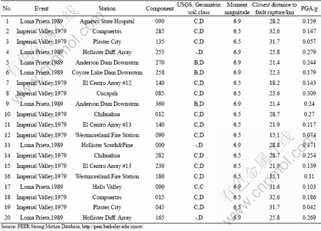
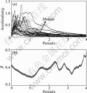
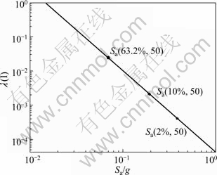
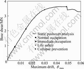
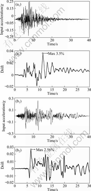
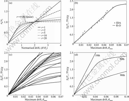
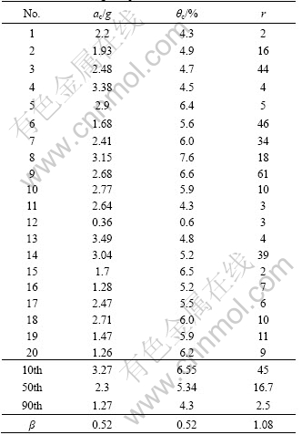
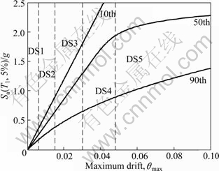
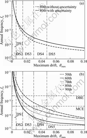
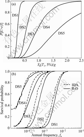
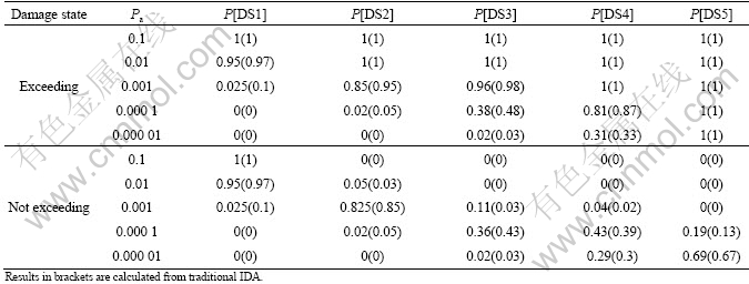
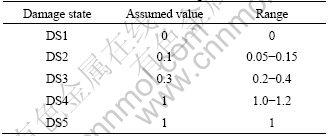
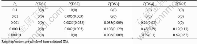
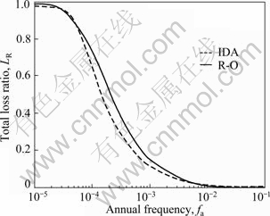
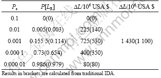
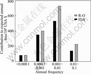
where fa is the annual frequency; i is the intensity measure; e is the engineering demand parameter; dm is the damage measure; dv is the decision variable (e.g. loss ratio, repair cost, and downtime); loss ratio (LR, Lr) is defined as the cost to repair a structure divided by the total replacement cost; G(x|y)=P(x 3 Case study of RC frame structure 3.1 Prototype details The generic methodology established so far is then applied to assessing the financial implications of earthquake hazard exposure to reinforced concrete frame structures. From this, an RC frame structure designed by ��Technical Specification for Concrete Structures of Tall Building�� [16] and ��Code for Seismic Design of Buildings�� [17] was adopted. The frame was designed as eight-degree fortification, site classification II, seismic design group 1. The natural period of the structure was approximately T1=1.08 s. The frame is considered to be located in a high seismic zone, where the design basis earthquake (DBE) is characterized by a peak ground acceleration of 0.3g. The reinforcement conditions of columns and beams and the elevation view of the structure are shown in Fig. 2(a). The beam reinforcement conditions are divided into four cases, and the column reinforcement conditions are divided into ten cases. The dead load and live load arrangement of the structure are shown in Figs. 2(b) and (c), respectively. The concrete strength grade of columns, beams and floor slabs is C30. The main reinforcement of columns and beams is HRB335, and the hooping is HPB235. The underlying story height is 3.9 m, and the remaining layer is 3 m. Cross section of beams is 300 mm��600 mm; that of columns is 700 mm��700 mm (1-4 layer) and 600 mm ��600 mm (5-8 layer). 3.2 Selection of ground motion records and earthquake-recurrence relation In order to perform IDA, a suite of ground motion records are needed. Due to the lack of large earthquakes in the region where the structure is located, there are insufficient regional ground motion records to use for the IDA. Therefore, a suite of ground motion records, previously used by VAMVATSIKOS and CORNELL [18] are adopted, which are presented in Table 1. These records, which are all recorded on firm soil, have magnitude and distance ranges of 6.5-6.9 and 15.1-31.7 km, respectively. The pseudo-acceleration spectra along with mean response spectrum of these records are exhibited in Fig. 3. Figure 3 also presents a plot of the lognormal standard deviation ��, always referred to as the dispersion, across the spectrum. Due to the consistent and relatively low values of ��, it is evident that Sa(T1, 5%) serves as an appropriate IM. According to Eqs. (1)-(3), values for k and k0 are determined to be 2.381 4 and 0.000 043 646. The hazard-recurrence curve is given in Fig. 4. It is shown that the points of Sa(63.2%, 50), Sa(10%, 50) and Sa(2%, 50) correspond to the spectral values of 63.2%, 10% and 2% of exceeding probability in 50 a (i.e. small earthquake, medium earthquake and large earthquake of the code), respectively. 3.3 Incremental dynamic analysis Prior to performing IDA, pushover analysis which is based on first-mode was conducted to the RC frame structure. It determined the values of quantitative indexes corresponding to different performance levels according to Ref. [19]. Figure 5 shows the base shear and maximum interstorey drift curve of the structure obtained by pushover analysis. The feature points on the curve correspond to the four overall damage limit states. In order to estimate structural performance under seismic loads, VAMVATSIKOS and CORNELL [20] proposed a computational-based methodology called incremental dynamic analysis (IDA). Conducting an IDA consists of running a series of inelastic dynamic time-history analyses at various levels of excitation, over a suite of earthquake records. This results in a matrix of data from which a probabilistic IM-EDP relationship is derived. Choosing an appropriate IM is an important step, since it can exert significant effect on the scatter of data. Current best practice for the first mode dominated structures is to use the 5% damped spectral acceleration at the fundamental period of the structure, Sa(T1, 5%), which has been shown to be relatively ��efficient�� and ��sufficient�� compared with PGA [21]. Fig. 2 Structural configurations: (a) Elevation model and reinforcement plans; (b) Dead load diagram; (c) Live load diagram Table 1 Earthquake records adopted for IDA [18] Fig. 3 Acceleration spectra (a) and lognormal standard deviation (b) Fig. 4 Hazard intensity-recurrence relations Fig. 5 Base shear and maximum drift curve of structure obtained by pushover analysis OpenSees [22], an inelastic dynamic time-history analysis program, was used to conduct the IDA. The Rayleigh elastic damping was taken as 5% of the critical one. Neither the soil�Cstructure interaction (i.e. firm soil site was assumed) nor the torsion and slab interaction effects were considered. Here, IDA was performed to generate the 5% damped spectral acceleration at the fundamental period of the structure, Sa(T1, 5%) versus the maximum interstorey drift, ��max relationship and the IDA results were quantitatively modeled and integrated into a probabilistic risk analysis procedure whereby the seismic intensity recurrence relationship (the seismic demand) was viewed with respect to the damage propensity of a specific frame structure (structural capacity). Confidence intervals and damage outcomes for given hazard intensity levels, such as the Design Basis Earthquake (DBE) or the Maximum Considered Earthquake (MCE), can then be evaluated. The 20 records were scaled between 0.1g and 2.5g with an increment of 0.1g, resulting in 500 separate analyses. The resulting plots by using multiple interpolation spline functions are given in Fig. 6. Also the dispersion (��) is shown in Fig. 6. It is evident that at lower level of IMs the dispersion is on the order of 0.25-0.3, whereas for the higher IMs where numerical instability occurs (meaning structural collapse), the level of dispersion increases to about 0.45�C0.55. Overall, the value of dispersion �� is relatively small. This partially justifies the selection of Sa(T1, 5%) as the intensity measure of seismic hazard. Fig. 6 Conventional IDA curves and dispersion From the IDA results, it is possible to identify those earthquakes that, in a probabilistic sense, inflict the most damage. It is of interest to scrutinize the structural response for a few selected ground motions corresponding to the desired performance bounds. Therefore, the acceleration and the response drift obtained from nonlinear time-history analysis for EQ5 and EQ14 are shown in Fig. 7. 3.4 Modeling of percentile IDA curves In previous studies, the IDA curves were usually derived by using multiple interpolation spline functions [20]. It is considered that such an approximation is cumbersome and not particularly useful for subsequent risk analysis [23]. Therefore, in this work, the Ramberg-Osgood (R-O) equation was explored as the most suitable functional relation. The R-O equation can be written in the following two forms: where K is the slope of IDA curve in initial proportional range; ac is the critical earthquake acceleration intensity that occurs at the onset of large drifts that subsequently lead to collapse; ��c=ac/K, is the critical value of EDP (drift); r is a constant. Fig. 7 Acceleration and response of drift obtained from nonlinear time-history analysis: (a) EQ5; (b) EQ14 The relationship and the significance of the three required control parameters (ac, r and either ��c or K) is examined, as shown in Fig. 8(a). With the increase of curvature parameter r, the curve tends toward a bilinear case (when r=��). If the input intensity, Sa(T1, 5%), is greater than the critical value, ac (i.e., ag>ac), then the response is ��>2��c and structural instability (i.e., collapse) is imminent. In Eq. (5), three control parameters (ac, r and either ��c or K) are estimated using a nonlinear least-square analysis on interpolated 10th, 50th and 90th percentile curves. The obtained values of the control parameters for different earthquakes are listed in Table 2. Figure 8(b) illustrates the fit between the actual IDA data points and the fitted R-O curve for EQ7 which shows a good agreement. Figures 8(c) and (d) show the R-O curves of all earthquakes and the fitted continuous smooth IDA curves representing the 10th, 50th and 90th percentile response demand. 3.5 Damage limit states Once the three percentile (10th, 50th and 90th percentile) lines have been generated as mentioned above, it is possible to determine the expected drift of the structure for an earthquake with a certain level of seismic intensity. According to the international best practice for seismic design, a dual level intensity approach is adopted: 1) A DBE represented by a 10% in 50-year ground motion (i.e. frequent earthquake of the code); 2) An MCE represented by a 2% in 50-year earthquake (i.e. rare earthquake of the code). Several damage limit-states can be defined on the IDA curves developed. In this work, the definitions of damage limit states are extended by performing pushover analysis (see Fig. 5) and definitions of damage states (DS) for the structure are listed in Table 3. Then, the defined damage states are assigned to the IDA percentile curves in Fig. 9. For Table 3 and Fig. 9, the first damage state (DS1) can be defined at the onset of damage as the computed yield drift (displacement) of the structure. The final damage state, DS5, occurs when the structure becomes dynamically unstable and collapses. This generally occurs when the lateral strength is exhausted as a result of longitudinal bar fracture from low cycle fatigue, or instability from the P-delta effect [23]. The other damage stages (DS2, DS3, and DS4) are more subjective in their definitions. It is suggested that the boundary that separates DS3 and DS4 can be defined at a level of drift where the structure would be deemed to have suffered irreparable damage such that the structure is not likely to perform its function as evidenced by: 1) excessive permanent drift at the end of the earthquake; 2) excessive level of damage to critical elements such as buckling of longitudinal reinforcing bars or the fracture of transverse hoops and/or longitudinal reinforcing bars. Finally, the boundary separating DS2 and DS3 should be defined as a level of damage which would cause temporary loss of function and immediate repairs are needed to restore the full functionality of the structure. This usually occurs when cracking of cover concrete is evident. At drifts below this boundary, damage (categorized as DS2) is considered to be slight and tolerable [15]. Fig. 8 Modeled IDA curves and generated response demand curves: (a) IDA modeling curves by Ramberg-Osgood equation; (b) Modeled IDA results with R-O relationship for EQ7; (c) Fitted IDA curves; (d) 10th, 50th and 90th percentile lines Table 2 R-O modeling and parameter identification Table 3 Damage states adapted from Pushover analysis and loss ratio assigned Fig. 9 Damage states assigned to IDA percentile curves 3.6 Drift hazard curve Equations (1) and (5) along with the information in Table 2, i.e. R-O parameters for the 50th percentile (median) IDA curve can be used to plot a full set of different percentile hazard recurrence-drift-damage curves. The developed IDA curves can be modified more elegantly by substituting the hazard-recurrence relationship [15]: where Note that the parameters ac, ��c and r depend on confidence intervals. According to MARTINEZ [24], for an appropriate closed-form of the cumulative lognormal probability density function, the confidence interval can be estimated by where ��C/D is the composite lognormal coefficient of variation; An example of the resulting drift hazard curves is presented graphically in Fig. 10(a), which can be used to estimate the annual frequency of exceeding a given damage state within a certain degree of confidence. It is well known that, in the performance-based assessment, sources of uncertainty are differentiated into aleatory sources and epistemic sources. The aleatory uncertainty reflects the variability due to random nature of ground motions (denoted as record-to-record variability). The epistemic uncertainty is mainly due to lack of knowledge about the building��s real model (inability to incorporate all elements that may contribute to lateral strength and stiffness in structural model) and real element properties (stiffness, strength, deterioration properties, etc) [25]. Simultaneously considering the effects of aleatory and epistemic uncertainties, it is necessary to use an integrated approach as suggested by KENNEDY et al [26]. The composite value of the lognormal coefficient of variation can be expressed as where ��C is the lognormal standard deviation for the capacity which arises as a result of the randomness of the material properties that affect strength; ��D is the lognormal standard deviation for the seismic demand which arises from record-to-record randomness in the earthquake ground motion suite; ��U is the lognormal dispersion parameter for model (i.e. epistemic) uncertainty. Fig. 10 Drift hazard curves: (a) Role of uncertainty; (b) Composite confidence interval curves with uncertainty Following the recommendations given by FEMA 350 [27], ��C and ��U are assumed to be 0.2 and 0.25, respectively. The original sets of percentile IDA curves (that have the dispersion ��D) can be modified by keeping the median (50th percentile) IDA curve intact and shifting away other curves such that the dispersion becomes ��C/D. The hazard recurrence curves that include both aleatory randomness and epistemic uncertainty can be plotted as the solid 80th percentile line for ��C/D= 0.5 in Fig. 10(a). As a comparison, it also gives the curve without considering uncertainty. For detailed assessment, additional confidence intervals can also be plotted with the 90th, 80th, 70th, 60th and 50th percentile curves, as shown in Fig. 10(b). From Fig. 10(a), it can be seen that the annual frequency considering uncertainty is larger than that without uncertainty consideration, which means that not considering the uncertainty in seismic financial assessment will underestimate the loss. Seen from Fig. 10(b), for a rare event, such as an MCE that has a 2% probability of recurrence in 50 year, it is evident that one can be at the least 80% confident of survival without collapse. 3.7 Risk assessment Through hazard curves (Fig. 10) and seismic fragility curves (Fig. 11(a)), the survival curves of the structure can be got. Figure 11(b) gives the probability of the defined damage states not being exceeded (computed by R-O equation) when earthquakes hit the structure (solid line). Based on the annual frequency or the return period of the earthquake, it shows the likelihood of the induced damage not crossing the limits of the five damage states. As also shown in Fig. 11(b), the hazard-survival curves are got from the conventional IDA results (dotted line). It can be seen from Fig. 11(b) that the survival probability calculated by conventional IDA curves under each damage state is larger than the modeling IDA curves (R-O equation). The information in Fig. 11(b) is also expressed in tabular form in Table 4. For example, the fourth row means that if an earthquake of annual frequency of 0.001 (i.e. return period of 1000 a) strikes the structure, the probability of DS1 not being exceeded is 2.5% for R-O equation and 10% for IDA results; the corresponding probabilities for other damage states (DS2, DS3, and DS4) are 85%, 96%, 100% for R-O equation and 95%, 98%, 100% for IDA results, respectively. Table 4 also presents the various probabilities of being in a given damage state. For example, the fourth row means that when an earthquake with an annual frequency of 0.001 strikes the structure, there is a 2.5% chance for R-O equation (10% for IDA) that the damage state will be DS1; 82.5%, 11% and 4% chance for R-O equation (85%, 3% and 2% for IDA) that the damage will be in the range of DS2, DS3 and DS4, respectively. Fig. 11 Quantitative risk assessment: (a) Seismic fragility curves; (b) Hazard-survival curves Table 4 Probabilities of exceeding and being in damage state 3.8 Annual financial risk The modified percentile IDA curves which consider uncertainty and randomness can be used to generate data points defining the probability of not exceeding a damage state given an annual frequency. This can be found by calculating the IM at each DS boundary for multiple percentile values of the distribution, and converting that IM to annual frequency. This relationship can be expressed by hazard-survival curves (see Fig. 11(b)). It is then possible to combine the multiple DSs into a single total loss curve. In discrete form, the expected annual loss (EAL, La) can be probabilistically calculated as where Pa(lr) is the annual frequency of loss ratio exceeding a given value lr, which can be obtained from the financial hazard curve. In order to calculate financial risk, one needs to know what the different damage states mean in terms of financial loss. The normalized cost is referred to as the loss ratio (LR) hereafter. The assumed values and possible ranges of loss ratios for different damage states are listed in Table 5. As DS1 is the pre-yielding damage state, neither damage nor repairs are expected. It follows that there are no financial losses, so the loss ratio for DS1 is assumed to be 0. DS2 is the post-yielding and minor-spalling damage state. It may require minor inspection and repairs at some stages. It is assumed herein that the loss ratio for DS2 will vary between 0.05 and 0.15, and a value of 0.1 is employed for further calculations. Likewise, DS3 refers to post-spalling and bar-bucking damage state. Repairs are expected to restore functionality. Accordingly, the loss ratio for DS3 may range from 0.2 to 0.4, and a representative value of 0.3 is adopted in the analysis. Extensive damage under DS4 generally means that although collapse has not occurred, the damage is too costly or uneconomic to repair, thus complete reconstruction is needed. Hence, the loss ratio for DS4 cannot be less than 1, and a value of 1 is used here. Finally, DS5 refers to collapse and requires total replacement. Obviously, the loss ratio for DS5 is 1. Table 5 Loss ratios for different damage states Then, the contribution of different damage states to the financial loss is estimated. Table 6 lists the probable loss ratios corresponding to different damage states when earthquakes with annual frequencies of 0.1, 0.01, 0.001, 0.000 1, and 0.000 01 strike. The values in Table 6 are the product of the probability of being in a given damage state (obtained from Table 4) in earthquakes of different annual frequencies and the assumed loss ratio for the corresponding damage state from Table 5. It can be expressed in terms of equation as follows: Seen from Table 6, DS1 does not incur any financial loss as it does not need any repair. Meanwhile, the financial loss incurred by earthquakes of 0.1 or higher annual frequency is also nil because such frequent events do not incur any damage. The total probable financial loss ratio due to earthquakes of a given frequency is the sum of the corresponding values for the five damage states. Figure 12 plots curve of the total probable loss ratio against the annual frequency of the earthquakes. Similarly, it also gives the curve obtained from conventional IDA results. Figure 12 gives information on what would be the financial loss if an earthquake of a given annual frequency strikes once. As the probability of being in more severe damage states are multiplied by higher loss ratios (as shown in Table 5, LR is higher for DS4 and DS5 than for others), the higher damage states contribute more to the probable loss although the likelihood of the earthquake-induced damage falling into these severer categories is not high. Table 6 Conditional probability of loss ratios Fig.12 Probable financial loss ratio against annual frequency The total probable financial loss for earthquakes of different frequencies is also reinterpreted in tabular form in Table 7. In the third column of Table 7, the expected annual loss (EAL) due to earthquakes of annual frequency within a range is calculated. In fact, the EAL is the area subtended by the economic hazard curve (Fig. 12) between two points on x-axis. Table 7 Annual expected loss ratio From Table 7, the calculated EAL is found to be USA $ 1 430 per USA $ 1 million gotten from R-O equation compared to USA $ 1 100 per USA $ 1 million gotten from conventional IDA results. This means that adopting conventional IDA curves (suggested by VAMVATSIKOS and CORNELL) to calculate the financial risk of the structure will underestimate the loss. The annual financial risk due to earthquakes of different frequency ranges is also depicted in Fig. 13. It is reasonable to assume that the earthquakes with annual frequencies smaller than 0.000 01 (return period of more than 10 000 year) will pose small financial risk and is hence negligible. Similarly, the financial risk caused by earthquakes with annual frequency between 0.01 and 0.1 (return period of less than 100 year) is relatively small either, as they are all frequent events. Fig.13 Annual financial risk of different frequency ranges As evident in Table 7 and Fig. 13, the total annual financial risk calculated by R-O equation (i.e. the financial risk posed by all possible earthquakes) amounts about 0.143% of the total damage cost (i.e. replacement cost). In other words, the expected annual financial loss is USA $ 1 430 per USA $ 1 million. And about 50% of this value corresponds to the risk posed by relatively frequent and modest size earthquakes with an annual frequency in the range between 0.01 and 0.001 (i.e. return periods between 100 and 1 000 year). The same situation exists in the conventional IDA results. 4 Conclusions 1) Incremental dynamic analysis (IDA) is an effective method of assessing seismic response in terms of a given engineering demand parameter (EDP). It can record the whole process of the structure from yield, damage until collapse, and provide basis for the next seismic financial risk assessment. Parameterizing the IDA results using Ramberg-Osgood (R-O) equation can get relatively accurate financial risk assessment. 2) The financial implications of damage can be expressed by EAL which can be expressed in terms of a loss ratio (LR) with respect to an earthquake ground motion that has an annual frequency fa. This parameter represents the median annual cost from seismic risk considering all possible earthquake scenarios. The computational IDA-EAL method will enable engineers to take into account the long-term financial implications in addition to the construction cost. Consequently, it will help the stakeholders to make informed decisions when choosing the final design for new buildings and a seismic retrofit option for existing buildings. 3) The EAL of the RC frame structure which is designed to a basis earthquake that has a 10% probability in 50 year with PGA of 0.3g is found to be in the order of USA $ 1 430 per USA $ 1 million of asset value which is larger than USA $ 1 100 per USA $ 1 million calculated by conventional IDA results. And about 50% of the EAL posed by relatively frequent and modest size earthquakes with an annual frequency in the range between 0.01 and 0.001. 4) There are several interrelationships involved in estimating the annual financial risk which has some limitations in assessing the financial loss of the proposed methodology: The natural hazard recurrence relationship is developed based on historical data; Sa(T1, 5%)-��max relationship is derived from the results of IDA; the maximum drifts corresponding to different damage states are assumed based on experience; the loss ratios for the different damage states are decided based on engineering judgment. References [1] CORNELL C A, JALAYER F, HAMBURGER R O. Probabilistic basis for 2000 SAC federal emergency management agency steel moment frame guidelines[J]. Journal of Structural Engineering, 2002, 128(4): 526-533. [2] KRAWINKLER H, MIRANDA E. Performance-based earthquake engineering in earthquake engineering: From engineering seismology to performance-based engineering [M]. Boca Raton: CRC Press, 2004. [3] AUGUSTI G, CIAMPOLI M. Performance-based design in risk assessment and reduction [J]. Probabilistic Engineering Mechanics, 2008, 23(4): 496-508. [4] BRADLEY B A, CUBRINOVSKI M, DHAKAL R P, MACRAE G A. Probabilistic seismic performance and loss assessment of a bridge-foundation-soil system [J]. Soil Dynamics and Earthquake Engineering, 2010, 30(5): 395-411. [5] ASLANI H, MIRANDA E. Probability-based seismic response analysis [J]. Engineering Structures, 2005, 279(8): 1151-1163. [6] BAKER J W. Probabilistic structural response assessment using vector-valued intensity measures [J]. Earthquake Engineering and Structural Dynamics, 2007, 36: 1861-1883. [7] RUIZ G J. Performance-based assessment of existing structures accounting for residual displacements [D]. Stanford, California: Stanford University, 2004. [8] KRAWINKLER H. A general approach to seismic performance assessment [C]// Proc International Conference on Advances and New Challenges in Earthquake Engineering Research, ICANCEER. Hong Kong, 2002: 173-180. [9] DEIERLEIN G G, KRAWINKLER H, CORNELL C A. A framework for performance-based earthquake engineering [C]// Pacific Conference on Earthquake Engineering. Christchurch, New Zealand, 2003: 140. [10] BAKER J W, CORNELL C A. Vector-valued ground motion intensity measure consisting of spectral acceleration and epsilon [J]. Earthquake Engineering and Structural Dynamics, 2005, 34(10): 1193-1217. [11] TOTHONG P, LUCO N. Probabilistic seismic demand analysis using advanced ground motion intensity measures [J]. Earthquake Engineering and Structural Dynamics, 2007, 36(13): 1837-1860. [12] ALAVI B, KRAWINKLER H. Behavior of moment-resisting frame structures subjected to near-fault ground motions [J]. Earthquake Engineering and Structural Dynamics, 2004, 33(6): 687-706. [13] LUCO N, CORNELL C A. Structure-specific scalar intensity measures for near-source and ordinary earthquake ground motions [J]. Earthquake Spectral, 2007, 23(2): 357-392. [14] BAKER J W, CORNELL C A. Vector-valued intensity measures for pulse-like near-fault ground motions [J]. Engineering Structures, 2008, 30: 1048-1057. [15] DHAKAL R P, MANDER J B. Financial risk assessment methodology for natural hazards [J]. Bulletin of the New Zealand Society of Earthquake Engineering, 2006, 39(2): 91-105. [16] JGJ 3��2002, Technical specification for concrete structures of tall building [S]. [17] GB 50011��2001, Code for seismic design of buildings [S]. [18] VAMVATSIKOS D, CORNELL C A. Developing efficient scalar and vector intensity measures for IDA capacity estimation by incorporating elastic spectral shape information [J]. Earthquake Engineering and Structural Dynamics, 2005, 34(13): 1573-1600. [19] ERBERIK M A, ELNASHAI A S. Fragility analysis of flat-slab structures [J]. Engineering Structures, 2004, 26: 937-948. [20] VAMVATSIKOS D, CORNELL C A. Incremental dynamic analysis [J]. Earthquake Engineering and Structural Dynamics, 2002, 31: 491-514. [21] SHOME N, CORNELL C A, BAZZURRO P, CARBALLO J E. Earthquakes, records, and nonlinear responses [J]. Earthquake Spectra, 1998, 14(3): 469-500. [22] OPENSEES. Open system for earthquake engineering simulation [EB/OL]. 2009, http://opensees.berkeley.edu. [23] MANDER J B, DHAKAL R P, MASHIKO N, SOLBERG K M. Incremental dynamic analysis applied to seismic financial risk assessment of bridges [J]. Engineering Structures, 2007, 29: 2662-2672. [24] MARTINEZ M E. Performance-based seismic design and probabilistic assessment of reinforced concrete moment resisting frame structures [D]. New Zealand: Department of Civil Engineering, University of Canterbury, 2002. [25] ZAREIAN F, KRAWINKLER H. Assessment of probability of collapse and design for collapse safety [J]. Earthquake Engineering and Structural Dynamics, 2007, 36(13): 1901-1914. [26] KENNEDY R P, CORNELL C A, CAMPBELL R D, KAPLAN S, PERLA H F. Probabilistic seismic safety study of an existing nuclear power plant [J]. Nuclear Engineering and Design, 1980, 59(2): 315-338. [27] Federal emergency management agency (FEMA). Recommended seismic design criteria for new steel moment-frame buildings [R]. Rep. No. FEMA-350. Washington (DC): SAC Joint Venture, 2000. (Edited by YANG Bing) Foundation item: Project(2011CB013804) supported by the National Basic Research Program of China; Project(50925828) supported by the National Natural Science Funds for Distinguished Young Scholars of China Received date: 2011-03-17; Accepted date: 2011-06-27 Corresponding author: ZHU Hong-ping, Professor, PhD; Tel: +86-27-87542631; E-mail: hpzhu@mail.hust.edu.cn

 (5)
(5)


 (6)
(6)![]() = Sa(T1, 5%), relevant to its return period;
= Sa(T1, 5%), relevant to its return period;![]() = Sa(T1, 5%), with a return period of 475 year (10% probability in 50 year); Tr is the return period; pa is the annual probability (pa=1/Tr); q is an exponent based on local seismicity. The value of q is 0.42 in this work.
= Sa(T1, 5%), with a return period of 475 year (10% probability in 50 year); Tr is the return period; pa is the annual probability (pa=1/Tr); q is an exponent based on local seismicity. The value of q is 0.42 in this work. (7)
(7)![]() is the median (50th percentile) of the distribution of variable x. Through Eq. (7), the value of the parameter xCI for a given confidence interval CI can be estimated by
is the median (50th percentile) of the distribution of variable x. Through Eq. (7), the value of the parameter xCI for a given confidence interval CI can be estimated by![]() (8)
(8)![]() (9)
(9)
![]() (10)
(10)
![]() (11)
(11)
Abstract: Engineering facilities subjected to natural hazards (such as winds and earthquakes) will result in risk when any designed system (i.e. capacity) will not be able to meet the performance required (i.e. demand). Risk might be expressed either as a likelihood of damage or potential financial loss. Engineers tend to make use of the former (i.e. damage). Nevertheless, other non-technical stakeholders cannot get useful information from damage. However, if financial risk is expressed on the basis of probable monetary loss, it will be easily understood by all. Therefore, it is necessary to develop methodologies which communicate the system capacity and demand to financial risk. Incremental dynamic analysis (IDA) was applied in a performance-based earthquake engineering context to do hazard analysis, structural analysis, damage analysis and loss analysis of a reinforced concrete (RC) frame structure. And the financial implications of risk were expressed by expected annual loss (EAL). The quantitative risk analysis proposed is applicable to any engineering facilities and any natural hazards. It is shown that the results from the IDA can be used to assess the overall financial risk exposure to earthquake hazard for a given constructed facility. The computational IDA-EAL method will enable engineers to take into account the long-term financial implications in addition to the construction cost. Consequently, it will help stakeholders make decisions.
