
J. Cent. South Univ. (2013) 20: 536-540
DOI: 10.1007/s11771-013-1516-9

Comparisons between unsteady sediment-transport modeling
Lahouari Benayada1, Mahmoud Hasbaia2
1. Department of Architecture, University of Sciences and Technology, PO Box 1505 El-M��Nouar, Algeria;
2. Department of hydraulics, University of M��Sila, PO Box 166 Ichebilia, Algeria
 Central South University Press and Springer-Verlag Berlin Heidelberg 2013
Abstract:
The comparative study between unsteady flow models in alluvial streams shows a chaotic residue as for the choices of a forecasting model. The difficulty resides in the choice of the expressions of friction resistance and sediment transport. Three types of mathematical models were selected. Models of type one and two are fairly general, but require a considerable number of boundary conditions, which related to each size range of sediments. It can be a handicap during rivers studies which are not very well followed in terms of experimental measurements. Also, the use of complex models is not always founded. But then, the model of type three requires a limited number of boundary conditions and solves only a system of three equations at each time step. It allows a considerable saving in calculating times.
Key words:
friction resistance; bed load; suspended load; mobile-bed modeling��
1 Introduction
The human interventions such as constructions of any installation or natural events such as the flood can considerably change the river��s profile. At the front of Cayenne��s mouth 40��107 m3 of mud was deposited in six years. During the flood of the Gange, excavations of 50 m were observed. Studies of loss storage capacity were conducted in many countries. Investigations of 66 dams, in USA, lead to the conclusion that 16% of capacity was lost in 22 years. In China, a study of 20 representative dams showed that 19% of the reservoir capacity was lost in 20 years. The capacity of Ghrib dam, in Algeria, has been reduced to 46% in 41 years. The capacity of small dams in Algeria fell down by 52% in over 40 years (1940�C1980). In Algeria, the life-span of dam is 30 years. Furthermore, we will quote the flood of three days in March 1974 when 3��107 t of sediment was drained in Algiers region.
Considering this magnitude, inquiring the aggradations and degradations in transient flow phenomenon remains necessary before any development project. In this work, our goal is not to make an exhaustive study of the question, but a critical thinking based on a comparative study of various existing models. For this work, we selected three types of mathematical models: model of type one, model of type two and model of type three. This choice is justified by the generality of the approach to the problem in these three models.
2 Governing equations and assumptions
Three governing equations describe unsteady open channel flow with movable boundary are as follows [1�C2].
1) flow-continuity equation:
 (1)
(1)
2��sediment-continuity equation:

 (2)
(2)
3) momentum equation:

 (3)
(3)
where A is the liquid flow area; Ae is the section of flow layer; Ac is the section of the bedload area; Af is the alluvial bed area; Cm is the average volumetric sediment concentration; Dx is the coefficient of dissemination of the concentration of the suspended materials; h is the flow depth; I is the bed slope; J is the friction slope; Pc is the porosity of bedload area; Pf is the bed-sediment porosity; Qes is the volumetric flow rate of sediment- water mixture; Qsc is the bedload transport rate; �� is the water-sediment mixture density; ��s is the sediment density; g is the gravitational acceleration; x is the distance; t is the time; Vs is the suspended material velocity.
The fundamental assumptions made in the derivation of these equations are: the classic one-dimensional De Saint Venant hypothesis for the liquid phase is invoked, and the densities ��e and ��s are supposed to be constants.
Two supplementary equations are necessary in order to solve the system of Eqs. (1), (2) and (3).
2.1 Friction resistance
In its most general form, the friction resistance can be written as [3�C5]
J(V, H, ��, ��s,��)=0 (4)
2.2 Sediment transport
The prediction of sediment transport is fraught with difficulties. A multitude of sediment transport predictors are available, but they give predictions that easily differ from one another by orders of magnitude [6]. In this regard, the synthesis of the comparative study, between bedload formulas, developed by Botcheva and Iocheva [7] is presented in table 1.
2.3 Model of type one
This model takes into account liquid-continuity equation, sediment-continuity equation and momentum equation [8]. The fundamental assumptions are:only bedload transport is considered, Ac/A<<1, the porosity Pf is constant, and  and
and  are negligible.
Consequently, the system of equations governing the fluid-sediment motion may be summarized as
 (5)
(5)
 (6)
(6)
 (7)
(7)
As shown in fig. 1, a sediment mixture is schematized as comprising several discrete size classes of material, where Fk symbolises the weight sediments of diameter upper than  in percentage. The grading curve is divided into K classes. Each class, limited by the diameters and
 , is represented by a single diameter dk. The last one can be evaluated, for example, starting from the geometric mean of the two limiting diameters of the involved class. The equilibrium value of the total bedload will be done starting from the bedload relating to each particle-size range and given by Eq. (4).
On the other hand, as presented in fig. 2, the bed is considered composed of three parts: mixed layer, underlying coats and original bed.
Table 1 Comparative synthesis between bedload formulas
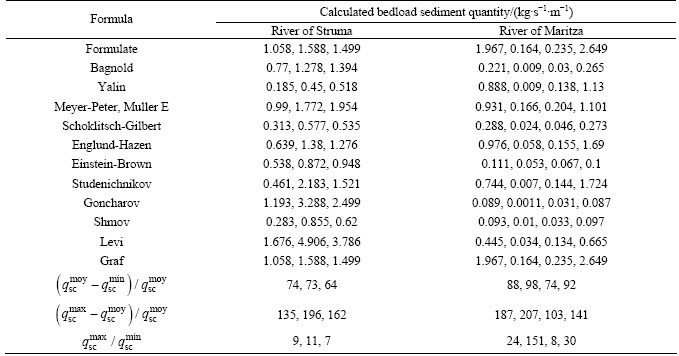
Fig. 1 Schematic representation of sediment mixture in model of type one
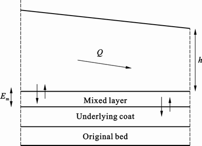
Fig. 2 Bedload modelling according to model type one
The mathematical concept of mixed layer, used by Karim and Kennedy [9], is used again here. This layer of variable thickness is at the upper level of the bed. So, the exchanges of materials are made at two levels, on one part, between this one and sediments in movement and on the other part, between this one and the sub-layers of the bottom.
The undercoats memorize the history of the bed composition. Their thicknesses are supposed to be constants. To follow the bed sediment mixture distribution, it is necessary to assess the flow of mass setting at stake into the mixed layer. It takes place from the writing of mass sediment balance sheet concerning each class size k within the mixed layer. Besides, this model takes spatial lag effects in bedload sediment transport into account.
After all, in this first type of model, the simulation of degradation of alluvial channel beds is then reduced to the resolution of (2K+3) equations: the flow-continuity equation, the sediment-continuity equation, the momentum equation, K spatial lag bedload sediments equations, K equations of bed composition. K+2 addition relations are required to solve the governing equations: Manning-Strickler equation for friction resistance, and K Meyer-Peter-Muller bedload sediments equations for each size class of sediment.
2.4 Model of type tow
This model takes into account bedload and suspended load sediments simultaneously [10]. This is made separately by introducing an exchange term between bedload and suspended load sediments. So, in addition to the hypotheses of the model of type one, the velocity of water and suspended sediments are considered to be equal. The balance sheet equations can be written in the following form:
 (8)
(8)
 (9)
(9)
 (10)
(10)
 (11)
(11)
where SS represents the exchange term between bedload and suspended load sediments. The latter one is evaluated by using spatial lag effects on suspended sediment transport.
This model takes into account spatial lag effects on bedload and suspended load sediments transport. By following the same path as before about the concept of mixed layer, in this model, we introduce a new term exchange in the sediment-continuity equation for each size class K. This expresses the exchange between the mixed layer and the suspended sediments. Finally, the problem comes back to solve (3k+3) equations: the flow-continuity equation, the sediment-continuity equation, the momentum equation, K spatial lag bedload sediments equations, K spatial lag suspended load sediments equations, and K equations of bed composition.
In this model, the (2K+2) addition relations are required to solve the governing equations: Manning-Strickler equation for friction resistance, a mixed layer thickness equation, K Meyer-Peter-Muller bedload sediments equations for each size class of sediments, and K equations linked to the transport capacity of suspended sediments for each size class.
The resolution is made in an uncoupled manner, in two stages: the first one solves (2K+3) equations; the second allows the evaluation of the suspended sediment concentrations.
2.5 Model of type three
In this model, the treatment of sediment mixtures is approached in a different way [11]. The flow variables are: total discharge, Q (Q=Qes+Qsc), flow depth h and bed elevation Zf. The majority of the hypotheses of the model of type two are considered. The bedload and suspended load sediment transport are examined according to an overview. The same balance sheet equations are considered, taking into account the flow-sediment-continuity equation in place of the sediment-continuity equation. The bedload and suspended load sediment transport are examined in a global manner. Consequently, the following system is got:
 (12)
(12)
 (13)
(13)
 (14)
(14)
where B is the width surface.
In this model, the grain-size distribution of the bed is examined differently. Indeed, the bed is considered composed of equal thickness layers to 2d90 as indicated in fig. 3. The model memorizes a maximum of 13 layers.
The layer being in contact with water is called active layer. if the aforementioned is eroded or filled, the one below or a new layer becomes active. At each time step, the sediment size distribution is updated according to a distribution chosen beforehand, expressed in weight percentage and shared in 13 classes defined in Table 2.
As the model does not take into account the lag effects on sediments transport, the study of sediment transport and bed form evolution is done in two steps. In the first stage, one solves the system formed by three equations of balance sheet, by considering a unique representative diameter of all the grain-size distribution. This solution allows evaluating the eroded section; In the second stage, the grain-size distribution is updated based on eroded section, where the flow celerity is compared with the critical celerity stemming from the diagram of Shields.
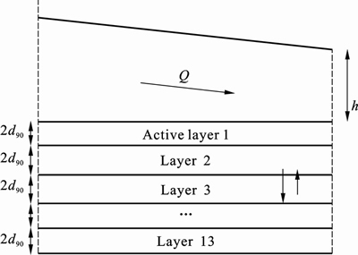
Fig. 3 Modelling of bed river according to model of type three
3 Comparative study
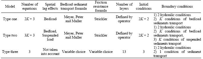
The model of type two represents an enrichment of the model of type one which takes into account only the bedload sediments. The introduction of the suspended load sediments is examined in a separate procedure. There are K characteristics related to grain-size distribution of suspended load, so K supplementary boundary conditions are required to solve the system as presented in table 3.
The consideration of the spatial lag modifies the nature of the equations originally hyperbolic. Its effect is translated by K characteristics of infinites celerity which propagate from upstream to downstream. These express the instantaneous transmission of information along the flow. The model of type three does not take into account the effects of the spatial lag, and the grain size distribution is updated at each time step. The problem is reduced to solve a system of three equations, therefore three boundary conditions are sufficient to find the solution.
Table 2 Size ranges used in model of type three
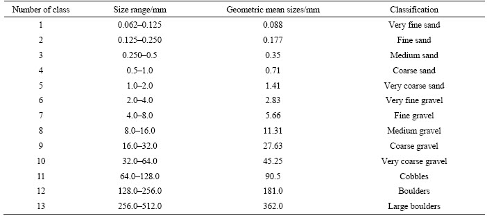
Table 3 Characteristics synthesis of three types of models
4 Conclusions
1) Modelling of aggradation and degradation of alluvial channel involves two types of equations: conservation laws written in any and all mathematical rigor, and semi-empirical equations, which express friction resistance and sediment transport. The major difficulty is related to the choice of these two semi-empirical equations relating to the case study.
2) Quantitative prediction of the resistance to fully turbulent flow in natural open channels is a problem of central importance in hydraulic and sedimentation engineering. On the other hand, the reliability of a mathematical model is strictly dependent upon the accuracy of the empirical equations used to evaluate the sediment transport. In fact, the sediment-transport evaluation is probably the major source of error that can affect the prediction of model.
3) Models of type one and two are fairly general, but require a considerable number of boundary conditions, which related to each size range of sediments. This can be a handicap during rivers�� studies which are not very well followed in terms of experimental measurements. Also, the use of complex models is not always founded. But then, the model of type three solves only a system of three equations at each time step, and it allows a considerable saving in calculating times.
4) Ultimately, the choice of prediction model is still a very sensitive issue. Indeed, the availability of experimental measures is important. On the other hand, the choice of friction resistance expressions and sediment transport is relatively important.
References
[1] Huang S L. Effect of using different sediment transport formulae and method of computing Manning��s roughness coefficient on numerical modelling of sediment transport [J]. Journal of Hydraulic research, 2007, 45(3): 347�C356.
[2] Papanicolaou A, Bdour A, Wicklein E. One-dimensional hydrodynamic/sediment transport model applicable to steep mountain streams [J]. Journal of Hydraulic Research, 2004, 42(4): 357�C375.
[3] Burguete J, Garcia-Navarro P, Murillo J, Garcia-Palacin I. Analysis of the friction term in the One-dimensional shallow-Water model [J]. Journal of Hydraulic Engineering, 2007, 133(9): 1048�C1063.
[4] Hu S, Abrahams A D. The effect of bed mobility on resistance to overland low [J]. Earth Surf Process, Landforms, 2005, 30: 1461�C1470.
[5] Morvan H, Knight D, Wright N, Tang X, Crossley A. The concept of roughness in fluvial hydraulics and its formulation in 1D, 2D and 3D numerical simulation models [J]. Journal of Hydraulic research, 2008, 46(2): 191�C208.
[6] Ben Slama E, Peron S, Belleudry P. TSAR: One-dimensional simulation of degradation of alluvial channel beds [C]// Hydrotechnical Symposium, Session No. 148. France: Hydrotechnical Society, 1993. (in French)
[7] Botcheva M M, Iocheva V D. Applicability of bed-load sediment formulas to natural Bulgarian river flows [R]. 21 ��me Congress AIRH, Canada, 1989: B331�CB337.
[8] Rahuel J L, Holly F M, Chollet J P, Belleudry P J, Yang G. Modeling of riverbed evolution for bedload sediment mixtures [J]. Journal of Hydraulic Engineering, 1989, 115(11): 1521�C1542.
[9] Karim M F, Kennedy J F. Computer-based predictors for sediment discharge and friction factor of alluvial streams [R]. IIHR, Report No. 242. University of Iowa City, USA, 1981.
[10] Yang G. Modeling of riverbed evolution for sediment mixtures [D]. University Joseph Fourrier, Grenoble I, France, 1989. (in French)
[11] Correia L R P, Krishappan B G, Graf W H. Fully coupled mobile boundary [J]. Journal of Hydraulic Engineering, 1992, 118(3): 476�C794.
(Edited by Yang Bing)
Received date: 2012�C02�C21; Accepted date: 2012�C09�C06
Corresponding author: Lahouari Benayada, Professor; Tel: +213-5-54120714; E-mail: benayada_lahouari@yahoo.fr
Abstract: The comparative study between unsteady flow models in alluvial streams shows a chaotic residue as for the choices of a forecasting model. The difficulty resides in the choice of the expressions of friction resistance and sediment transport. Three types of mathematical models were selected. Models of type one and two are fairly general, but require a considerable number of boundary conditions, which related to each size range of sediments. It can be a handicap during rivers studies which are not very well followed in terms of experimental measurements. Also, the use of complex models is not always founded. But then, the model of type three requires a limited number of boundary conditions and solves only a system of three equations at each time step. It allows a considerable saving in calculating times.
