J. Cent. South Univ. (2017) 24: 1696-1702

DOI: 10.1007/s11771-017-3576-8

LU Shao-fei(陆绍飞)¹, WU Heng(伍恒)², Eduardo Colmenares³, LIU Xu-chong(刘绪崇)⁴

1. College of Computer Science and Electronic Engineering, Hunan University, Changsha 410082, China;

2. Department of Computer Science, Texas Tech University, Lubbock 79409, USA;

3. Department of Computer Science, Midwestern State University, Wichita Falls 76308, USA;

Central South University Press and Springer-Verlag Berlin Heidelberg 2017

Abstract:

Direct dynamics simulations are a useful and general approach for studying the atomistic properties of complex chemical systems because they do not require fitting an analytic potential energy function. Hessian-based predictor-corrector integrators are a widely used approach for calculating the trajectories of moving atoms in direct dynamics simulations. We employ a monodromy matrix to propose a tool for evaluating the accuracy of integrators in the trajectory calculation. We choose a general velocity Verlet as a different object. We also simulate molecular with hydrogen(CO₂) and molecular with hydrogen (H₂O) motions. Comparing the eigenvalues of monodromy matrix, many simulations show that Hessian-based predictor-corrector integrators perform well for Hessian updates and non-Hessian updates. Hessian-based predictor-corrector integrator with Hessian update has a strong performance in the H₂O simulations. Hessian-based predictor-corrector integrator with Hessian update has a strong performance when the integrating step of the velocity Verlet approach is tripled for the predicting step. In the CO₂ simulations, a strong performance occurs when the integrating step is a multiple of five.

Key words:

monodromy matrix; eigenvalue; Hessian-based predictor-corrector; velocity Verlet；

1 Introduction

Classical chemical and molecular dynamics simulations are widely employed to study molecular processes [1-3]. Because the computational cost of Hessian models increases rapidly as dimension increases, an approximation to the Hessian for some integrations makes classical trajectory calculation more practical. The monodromy matrix is used as a test tool because of its special calculation features. It is used to check not only whether position and moments are canonically evolved, but also whether integration approximations are accurate.

The tradition approach uses a fitted analytic potential energy surface(PES) or a model force field to perform a classical dynamics simulation. Unfortunately, this is not an easy task because it is difficult to assess the accuracy of the integration of trajectory.

Direct dynamics is more general approach for classical dynamics simulations, in which the potential and its derivatives are obtained directly “on-the-fly” from an electronic structure theory. Direct dynamics [4-12] has become an important simulation tool for an increasing number of problems in fields as diverse as chemistry, materials science and biology. Despite the fact that the Hessian may be directly provided by some electronic structure theories, the computational cost of a Hessian calculation for trajectory integration at each time-step of a direct dynamics simulation is sometimes unacceptably high. To overcome this problem, some studies proposed different Hessian update approaches [13, 14]. Therefore, it is important to find a robust and trustworthy tool for estimating the accuracy of the trajectory integration. The monodromy matrix calculation becomes extraordinarily important for this reason [15].

Using the semi-classical dynamics simulations for CO₂ and H₂O on VENUS/NWChem, our work compares the monotromy for the Hessian-based predictor-corrector integrators and the monodromy matrix for velocity Verlet integrator. Experiment data show that for some semi-classical dynamics simulations, monitoring the monodromy matrix eigenvalues is essential for establishing the accuracy of trajectory integrators.

2 Methodology

The numerical accuracy of a classical trajectory time integration is usually determined by monitoring energy conservation. However, a different approach may be taken in order to see how a small perturbation introduced by a numerical approximation is propagated one time. We employ the equations of motion of the monodromy matrix, focusing on their interpretation in terms of the separation of nearby classical trajectories. When two classical trajectories are ifinitesimally close to each other at the starting phase space point and then evolve with time t, their phases space separation is given by

                (1)

where (δp₀, δq₀) are the initial separations in phase space and (δp_t, δq_t) are the final separation ones. Equation (1) can be written in a more compact form by introducing the (stability) monodromy matrix [16]

                           (2)

where the block element m_pq is

                 (3)

and the partial derivative are the initial positions for each momentum at time t; N is the number of degrees of freedom, and the dimension of the monodromy matrix is 2N×2N. By integrating Eq. (2) into Eq. (1), the final phase space separation becomes:

                    (4)

According to the classical Hamiltonian for N degrees of freedom, we have:

           (5)

From Eq. (4) and Eq. (5), one obtains the following equations:

                            (6)

                            (7)

where Hamilton’s equations have been employed. If one considers a deviation δq, the corresponding Hamiltonian deviation is

                   (8)

Then, the right-hand side of Eq. (6) is

                           (9)

and Eq. (6) becomes

                           (10)

In the same fashion, Eq. (7) becomes the following equality:

                     (11)

Assuming the same mass m for each degree of freedom without a loss of generality, the momenta and positions separations can be written as

                       (12)

where Eq. (4) has been used and

                        (13)

If Eq. (4) is derived with respect to time as

                       (14)

Equation (4) is equated to Eq. (12), then the time evolution of the monodromy matrix becomes:

                          (15)

where the initial condition is the identity matrix from the definition of Eq. (2). Key properties of the monodromy matrix are that its determinant is unity at the initial time and that determinant value is preserved under classical time evolution. The first property is easily verified by Eqs. (2) and (3). The second may be proven by either recognizing that the determinant of the monodromy matrix may be viewed as a Jacobian for the change of variables (p(t), q(t))→(p(t+dt), q(t+dt)) or a phase space area. The conservation of the determinant is equivalent to stating that the trajectory is canonically integrated. This property is a direct consequence of Liouville’s theorem.

In order to integrate the classical trajectories and the monodromy matrix M in Eq. (15), we employed symplectic algorithms, such as the second order velocity Verlet method and the Hessian-based predictor-corrector integrator. An explicit symplectic integrator form Eq. (15) is given by

              (16)

              (17)

                (18)

                (19)

where k=1, 2, …, m; m is the symplectic integrator order; The coefficients a_k and b_k are chosen in order to satisfy the integrator time-reversibility and some specified dynamics accuracy criteria of the order O(Δtⁿ) in Δt, with n ≤ m. A list of coefficients is given in Ref. [17], and V(q_k) and T(p_k) are respectively the potential and the kinetic energy at step k. If Eq. (16) is substituted into the right-hand side of Eqs. (18) and (17) into the right-hand side of Eq. (19), then the monodromy matrix at the kth integration step can be expressed in terms of the monodromy matrix at the (k-1)th step as

                        (20)

where I is the N×N identity matrix, and N is the number of degrees of freedom. Remember that det(A·B·C)=det(A) det(B) det(C) and rewrite Eq. (20) as

      (21)

Assuming that det(M^k-1)=1, Eq. (21) implies that the monodromy determinant value of unity is preserved for all time steps. Moreover, Eq. (21) shows that the algorithm is symplectic for any choice of the coefficients a_k and b_k and any form of the kinetic (²T(p_k))/(p_k²) and potential

Our understanding is that the deviations of det(M) from unity obtained for H₂O and CO₂ are caused by round-off errors resulting from large monodromy elements. The large values for these elements here are not necessarily produced by chaos but by the approximations applied to calculate the Hessian matrix.

To see qualitatively how monodromy elements can become exponentially larger, it is convenient to define the modified, but essentially equivalent, monodromy matrix:

                       (22)

where P=N^-1/2p, Q=N^1/2q, and N is the diagonal matrix of atomic masses. Then, M′ obeys

                           (23)

where

                              (24)

and H is the mass-scaled Hessian matrix calculated at q_k with elements:

                      (25)

For Δ_t is short enough, and H is almost constant, the solution of this equation is:

     (26)

where the diagonal matrix Λ contains the eigenvalues and the matrix U contains the eigenvectors of L. The diagonal elements λ_j of Λ are obtained by solving the secular equation:

                             (27)

Due to the simple block form of L, this equation can be expressed in terms of N-dimensional determinants as

                            (28)

which shows that the eigenvalues are given by

                                 (29)

where ω_j are the frequencies of the local normal mode coordinates.

According to the above derivation, we can detect any inaccuracies in the numerical integration of the classical equations of motion by calculating the determinant of this matrix at each time step. In particular, while the accuracy of the momenta and coordinates may be monitored from the energy conservation, the accuracy of Hessian matrix can be monitored by calculating the evolution of the monodromy matrix according to Eq. (16) and determining any deviation of the determinant from unity. The Hessian is part of the monodromy matrix time evolution, as shown by Eq. (13) and (16). If the numerical approximation of the Hessian is poor, then the determinant of the monodromy matrix will quickly deviate from unity.

3 Numerical tests

In testing, starting with time step K=0 Newton’s equation of motion is solved by calculating the positions and velocities of time step K+1 from time step K. In each time step, the inter-atomic forces are needed. Newton’s equation of motion is m(d²x/dt²)=F, where x is atom position, m means the mass of atom and F shows force that atom receives. F is equal to the potential energy gradient but in an opposite direction, so (d²x/dt²)=-G(x)/m. Here, the monodromy matrix evolution equation will be solved with initial condition

The Hessian-based integrator actually solves Newton’s equation of motion using the velocity Verlet integrator but on a constructed local potential energy surface(PES). In order to reduce ab initio electronic structure calculations, the Hessian-based integrator calculates the ab initio gradient and Hessian once every N steps, and in the remaining N-1 steps, the gradient needed by the velocity Verlet is approximated. The velocity Verlet employs Eq. (30) to integrate the trajectory, where M is the quality vector:

     (30)

The Hessian-based predictor-corrector algorithm has a prediction and a correction (see Fig. 1) for each time step. Let X₀ be the initial position, E₀, G₀, H₀, be the potential energy, and gradient and Hessian at X₀, respectively.

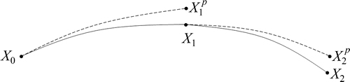
Fig.1 Hessian-based predictor-corrector algorithm at the first and second time steps (In the prediction, a trajectory is integrated from X₀ towhere the gradient of the potential energy is approximated by the Taylor expansion G(X)=G₀+ H₀(X-X₀). For the correction, the energy and its gradient and Hessian are first computed at and a trajectory is re-calculated from X₀ to X₁ using velocity Verlet, where the gradient of the position is provided by a fifth-order approximation using six pieces of potential energy information, three at X₀ (i.e. energy, gradient and Hessian) and three at )

Next, how does one update monodromy in Hessian-based predictor-corrector algorithm? Since the purpose of the predicted trajectory is to locate the point to help constructing an accurate local PES for the calculation of the corrected trajectory, monodromy needs to be calculated only on the corrected trajectory in each time step of the Hessian integrator, e.g. the Kth time step. Monodromy matrix is initialized to the identity matrix at X₀, but not at X_K for K≥1. In each time step Δt of the Hessian-based integrator, the velocity Verlet is used to calculate the corrected trajectory, where the time step Δt_vv of the velocity Verlet is much smaller than the time step Δt of the Hessian-based integrator. Monodromy matrix is to be calculated at each Verlet time step.

For the Hessian-base velocity Verlet integrator, the gradient is needed at the beginning and end of each time velocity Verlet step. These gradients are approximated from a 5th order high-dimensional interpolation. To calculate the monodromy matrix on the corrected trajectory with the velocity Verlet, Hessian is needed at the beginning and end of each Verlet time step. These Hessians are to be approximated using a Hessian update scheme.

Finally, how to approximate the Hessian for monodromy matrix calculation? At X_K, Hessian is needed for calculating the monodromy matrix but Hessian is not calculated at X_K in the Hessian-based integrator, but calculated at So, Hessian has to be approximated at X_K using the Hessian at Note that in the Hessian-based integrator, the Hessian at may also be approximated using Hessian update. But from the code writing perspective for adding monodromy calculation, it doesn’t matter if Hessian at is ab initio or approximated. After Hessian is approximated at X_K using the Hessian at in subsequent velocity Verlet steps in the Kth tie step of the Hessian integrator, the Hessian update at the ith Verlet time step is to use the Hessian at the (i–1)th Verlet time step for the update. In order to approximate the Hessian of the i-th Verlet time step in the Kth time step of the Hessian-based integrator, integration requires gradient at Hessian and gradient at of the (i–1)th Verlet step. The and are calculated by the Hessian integrator using the 5th order interpolation.

Direct dynamics simulations were performed with VENUS [18, 19] interfaced with NWCHEM [20]. Using a development version of the VENUS/NWChem package, simulations were performed with the monodromy matrix calculated at each time step. Simulations were performed for H₂O and CO₂, using B3LYP/cc-pVDZ theory. The Hessian is calculated directly in NWChem by an “analytic” linear algebra algorithm. The trajectories were calculated using Cartesian coordinates.

Figure 2 shows the simulation with Hessian update for CO₂. For Hessian-based predictor-corrector integration, the prediction step is 15 a.u.(1 a.u.= 2.418884×10^-17 s); while for Velocity Verlet integration, the time step is 10 a.u. The ab initio Hessian is calculated once in every 5 time steps. x label is time step, y label means the logarithm of the absolute for 1 minus eignvalue of each monodromy matrix element.

Figure 3 shows the simulation with Hessian update for H₂O. For Hessian-based predictor-corrector integration, the prediction step is 30 a.u.(a.u.= 2.418884×10^-17 s); while for velocity Verlet integration, the time step is 10 a.u. The ab initio Hessian is calculated once in every 5 time steps. x label is time step and y label means the logarithm of the absolute for 1 minus eignvalue of each monodromy matrix element.

According to simulation data, Hessian-based predictor-corrector integration performs well for CO₂ and H₂O when prediction step is 15 a.u. The green lines almost overlap the red lines for non-Hessian update or Hessian update. While the step is 10 a.u. for the velocity Verlet integration approach. For H₂O simulation, it still is well for Hessian-based predictor-corrector with Hessian update when prediction step is 30 a.u., three times time step of velocity Verlet integration approach. Furthermore, Hessian-based predictor-corrector without Hessian update performs well when prediction step is 30 a.u., three times time step of velocity Verlet integration approach.

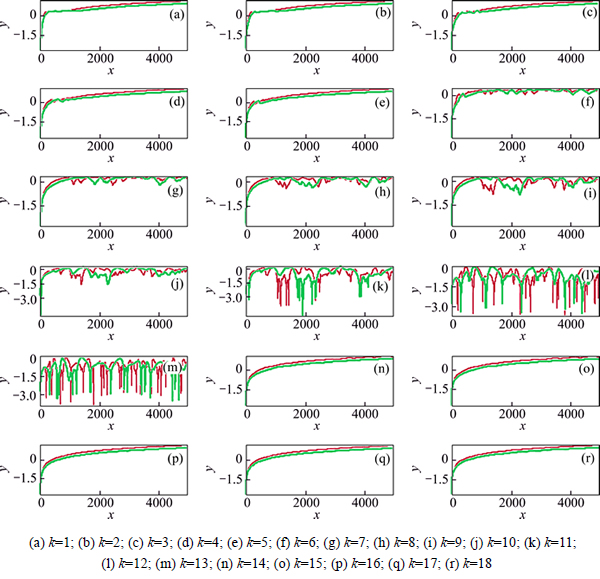
Fig. 2 Comparison of logarithm of eignvalue of each monodromy matrix element for CO₂ dynamics plotted step time (The red line is Hessian-based Predictor-Corrector integration with Hessian update and the green line is for velocity Verlet integration with Hessian update method. k is the ID of eignvalue of the monodromy matrix element. x label is step and y label is for lg(absolute(1-eignvalue))

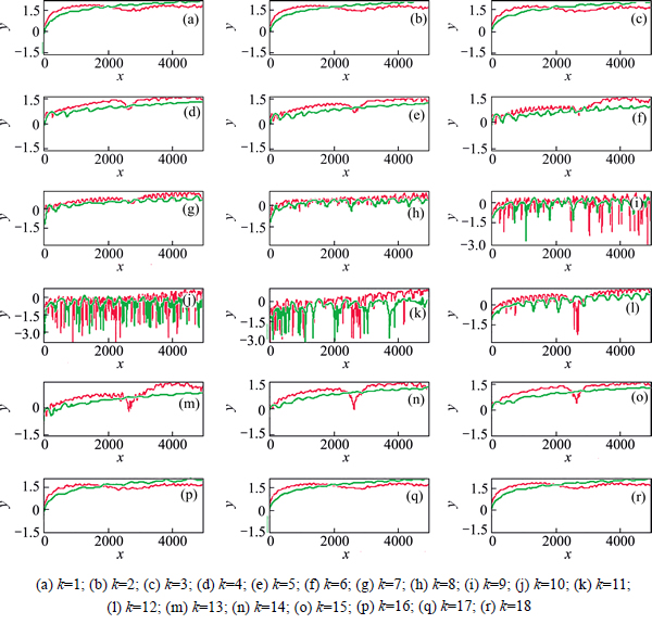
Fig. 3 Comparison of logarithm of eignvalue of each monodromy matrix element for H₂O dynamics plotted step time (The red line is Hessian-based predictor-corrector integration with Hessian update and the green line is for velocity Verlet integration with Hessian update method. k is the ID of eignvalue of the monodromy matrix element. x label is step and y label for lg(absolute(1-eignvalue))

4 Conclusions

Our works use monodromy matrix to compare the Hessian-based predictor corrector integrations with the velocity Verlet method on CO₂ and H₂O direct dynamics simulations. In the first simulations, monodromy matrix was calculated in the correct phase, while it was executed during trajectory integration in the second simulations. It is verified that the Hessian-based predictor-corrector integrations with Hessian update or non-Hessian update perform equally well, similar with velocity Verlet integration for CO₂ and H₂O simulations. It is obvious that the first is faster than the second under the same integration accuracy.

In the future, we will study the new predictor-corrector algorithms to reduce the computation time of Hessian under the premise of guaranteeing the precision based on date reusing and GPU. Deep learning can also be used to predict atomic trajectories in direct dynamics simulation. Simultaneously, monodromy matrix is used to verify the calculation accuracy for the new algorithms.

Acknowledgement

The authors thank the Chemdynm cluster at the Department of Chemistry & Biochemistry, Texas Tech University. The authors also thank Dr. Yu Zhuang and Bill Hase for their help.

References

[1] BUNKER D L. Classical trajectory methods [J]. Methods Comput Phys, 1971, 10(1): 287-325.

[2] PESLHERBE G H, WANG H, HASE W L. Monte Carlo sampling for classical trajectory simulations[J]. Adv Chem Phys, 1999, 105(1): 171-201.

[3] ALLEN M D, TILDESLEY D J. Computer simulation of liquids [M]. NY: Oxford Press, 1987.

[4] VOTH G A. Computer simulation of proton solvation and transport in aqueous and biomolecular systems [J]. Acc Chem Res, 2006, 39(1): 143-150.

[5] SUN L, HASE W L. Born-Oppenheimer direct dynamics classical trajectory simulations [J]. Rev Comput Chem, 2003, 19(1): 79-146.

[6] MARX D, HUTTER J. Ab initio molecular dynamics: Theory and implementation [C]// Modern Methods and Algorithms of Quantum Chemistry. Julich, Germany: John von Neumann Institute for Computing, 2000: 329-477.

[7] HERBERT J M, HEAD-GORDON M. Accelerated, energy- conserving Born–Oppenheimer molecular dynamicsviaFock matrix extrapolation [J]. Phys Chem Chem Phys, 2005, 7(1): 3269-3275.

[8] LI X C, TULLY J C, SCHLEGEL H B, FRISCH M J. Ab inito Ehrenfest dynamics [J]. J Chem Phys, 2005, 123(1): 084106.

[9] ISBORN C M, LI X, TULLY J C. Time-dependent density functional theory Ehrenfest dynamics: Collisions between atomic oxygen and graphite clusters [J]. J Chem Phys, 2007, 126(1): 134307.

[10] WU Heng, LU Shao-fei, ZUO Qin-wen, COLMENARES E. A high accuracy computing reduction algorithm based on data reuse for direct dynamics simulations [C]// The 2016 International Conference on Computational Science and Computational Intelligence (CSCI'16). Las Vegas, USA: IEEE, 2016: 1243-1247.

[11] WU Heng, LU Shao-fei, ZHU Ning-jia, LIU Jia-lin, COLMENARES E. A high order predictor-corrector integration algorithm for first principle chemical dynamics simulations [J]. Journal of Theoretical and Computational Chemistry, 2016, 15(1): 1-12.

[12] LIU Xu-chong, ZHANG Da-fang, HENG Gong, WU Heng. The comparative of a family of high order predictor-corrector algorithms for first principle chemical dynamics simulation [J]. International Journal of Enhanced Research in Science, Technology & Engineering, 2015, 4(10): 65-75.

[13] WU H, RANHMAN M, WANG J, LOURDERAJ U, HASE W L, ZHUANG Y. Higher-accuracy schemes for approximating the Hessian from electronic structure calculations in chemical dynamics simulations [J]. J Chem Phys, 2010, 133(1): 074101.

[14] HRATCHIAN H P, SCHLEGELH B. Using Hessian updating to increase the efficiency of a Hessian based predictor-corrector reaction path following method [J]. J Chem Theory Comput,2005,1(1): 61-69

[15] SCHLEGEL H B. Geometry optimization [J]. Wiley Interdisciplinary Reviews: Computational Molecular Science, 2011, 1(5): 790-809.

[16] WU Heng, LU Shao-fei. Evaluating the accuracy of a third order of a third order Hssian-based predictor-corrector integrator [C]// The 30th European Simulation and Modelling Conference. Las Palmas, Spain: EUROSES, 2016: 275-278.

[17] GUTZWILLER M C. Chaos in classical and quantum mechanics [M]. New York: Springer-Verlag, 1991: 1-29.

[18] ODELL A, DELIN A, JOHANSSON B, BOCK N, CHALLACOMBE M, NIKLASSON A M N. Higher-order symplectic integration in Born–Oppenheimer molecular dynamics [J]. J Chem Phys, 2009, 131(1): 244106.

[19] HU X, HASE W L, PIRRAGLIA T. Vectorization of the general Monte Carlo classical trajectory program VENUS [J]. J Comput Chem 1991, 12(1): 1014-1024.

[20] VALIEV M, BYLASKA E J, WANG D, NIEPLOCHA J, APRA E, WINDUS T L, DEJONGW A. NWChem: A comprehensive and scalable open-source solution for large scale molecular simulations [J]. Comput Phys Commun, 2010, 181(1): 1477-1489.

(Edited by YANG Hua)

Cite this article as:

LU Shao-fei, WU Heng, Eduardo Colmenares, LIU Xu-chong. Evaluating accuracy of Hessian- based predictor-corrector integrators [J]. Journal of Central South University, 2017, 24(7): 1696-1702.

Foundation item: Project(2016JJ2029) supported by Hunan Provincial Natural Science Foundation of China; Project(2016WLZC014) supported by the Open Research Fund of Hunan Provincial Key Laboratory of Network Investigational Technology; Project(2015HNWLFZ059) supported by the Open Research Fund of Key Laboratory of Network Crime Investigation of Hunan Provincial Colleges, China

Received date: 2016-08-03; Accepted date: 2017-01-08

Corresponding author: WU Heng, PhD Candidate; Tel: +86-731-88821974; E-mail: heng05.wu@ttu.edu

Abstract: Direct dynamics simulations are a useful and general approach for studying the atomistic properties of complex chemical systems because they do not require fitting an analytic potential energy function. Hessian-based predictor-corrector integrators are a widely used approach for calculating the trajectories of moving atoms in direct dynamics simulations. We employ a monodromy matrix to propose a tool for evaluating the accuracy of integrators in the trajectory calculation. We choose a general velocity Verlet as a different object. We also simulate molecular with hydrogen(CO₂) and molecular with hydrogen (H₂O) motions. Comparing the eigenvalues of monodromy matrix, many simulations show that Hessian-based predictor-corrector integrators perform well for Hessian updates and non-Hessian updates. Hessian-based predictor-corrector integrator with Hessian update has a strong performance in the H₂O simulations. Hessian-based predictor-corrector integrator with Hessian update has a strong performance when the integrating step of the velocity Verlet approach is tripled for the predicting step. In the CO₂ simulations, a strong performance occurs when the integrating step is a multiple of five.