J. Cent. South Univ. Technol. (2010) 17: 863-867

DOI: 10.1007/s11771-010-0568-3

Nonlinear combined forecasting model based on fuzzy adaptive variable weight and its application

JIANG Ai-hua(蒋爱华)¹, MEI Chi(梅炽)¹, E Jia-qiang(鄂加强)², SHI Zhang-ming(时章明)³

1. School of Energy Science and Engineering, Central South University, Changsha 410083, China;

2. College of Mechanical and Automotive Engineering, Hunan University, Changsha 410082, China;

3. Hunan Research Center of Energy-Saving Evaluation Technology, Central South University,

Changsha 410083, China

? Central South University Press and Springer-Verlag Berlin Heidelberg 2010

Key words:

nonlinear combined forecasting; nonlinear time series; method of fuzzy adaptive variable weight; relative error; adaptive control coefficient；

1 Introduction

For complex industrial systems with complicated inner configurations, a fairly large number of impact factors and evaluation indexes were partly shown when they were simulated, forecasted and controlled, and the forecasting values of the complex industry systems were made based on sole forecasting models or some partial factors and indexes for their input and output [1-5]. During the last ten years, a series of research results on combined forecasting models and methods have been acquired. For example, CHENG et al [6] proposed a novel method that incorporated trend-weighting into the fuzzy time-series models to explore the extent to which the innovation diffusion of information and communication technologies products could be adequately described by the proposed procedure. AGAMI et al [7] introduced a new approach for constructing trend impact analysis by using a dynamic forecasting model based on neural networks and enhancing the trend impact analysis prediction process. It was expected that such a dynamic mechanism would produce more robust and reliable forecasts. KOMORN?K et al [8] provided intuitive justification for the application of nonlinear two-regime models for modeling and forecasting of time series, and the forecasting performance of several nonlinear time series models was compared with respect to their capabilities of forecasting monthly and seasonal flows of the Tatry alpine mountain region in Slovakia.

On the contrary, the forecasting precision and simulated evaluation indexes of the complex industry systems will be enhanced by using many different forecasting models based on effective combined methods. And some new ideas to combine many different forecasting models were proposed from combined forecasting methods [9-12].

The models of determining combined weight coefficients were extensively established, but most of these researches were concentrated on studying various fixed weights in combined forecasting methods [13-14].

In Ref.[14], an algorithm was proposed to convexly combine the models for better performances of forecasting and the weights were sequentially updated after each additional observation. Simulations and real data examples were used to compare the performance of the approach with model selection methods.

Very limited researches were done based on variable weights [12, 15]. Therefore, in this work, a new nonlinear combined forecasting model was established based on the fuzzy adaptive variable weight.

2 Nonlinear combined forecasting model based on fuzzy adaptive variable weight

In the combined forecasting process, the determination of weight coefficients of combined models is vital. If weight coefficients are determined, the information from different forecasting methods will be synthesized in deed and the goal of enhancing forecasting precision will also come true.

Let the number of forecasting methods be n (n＞2) for some forecasting problems of nonlinear time series in complex industry processes. Their fuzzy control factors include relative error e_j(i) from the jth forecasting method at time i, and tendency c_j(i) of the forecasted object at time i, e_j(i) and c_j(i) are defined as

                           (1)

                    (2)

where j=1, 2, …, n; i＝1, 2, …, k, k is decided from the specific forecasting object and is equal to a certain value; y(i) is a true value at time i; and f_j (i) is the forecasting value from the jth forecasting method at time i.

2.1 Fuzzy controller

The fuzz process of relative error e_j(i) can be expressed as follows.

Firstly, a continuous area of [-1, 1] was divided into some sections, of which each was expressed as a discrete point. Let e_j(i) change in the area of [-1, 1], then, discrete area X about e_j(i) was gotten. Furthermore, A_k (k=1, …, 5) was used to express five semantic variables of relative errors e_j(i) as listed in Table 1.

Table 1 Corresponding semantic value in discrete area about forecasting values of relative errors

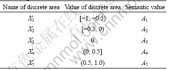
But in actual forecasting process, tendency c_j(i) of the forecasted object at time i will not always change in the area of [-1, 1], and maybe sometimes change in the area of [-M, M] (M, which is decided from the specific forecasting object, is a positive integer), therefore, the following formula can be used to translate tendency c_j(i) in the area of [-M, M] into variable c′_j(i) in the area of [-1, 1].

                              (3)

Furthermore, the discrete area about weigh l_j(i) from the jth forecasting method was changed in the range of [-1, 1] and the corresponding semantic value was gotten.

Let E denote the error between forecasting value from the jth forecasting method at time i and the true value at time i, C express the tendency rate of the forecasted value from the jth forecasting method at time i to true value at time i, and  express the fuzzy weight from the jth forecasting method at time i to true value at time i, then a control rule can be established as follows:

if E=e_j(i) and C=c′_j(i), then K_ij=k′_j (i)

Therefore, a fuzzy controller with double input parameters (e_j(i), c′_j(i)) and single output parameter (K_ij) was designed. Afterwards, output parameter (K_ij), namely the fuzzy weight, was adjudged by using the fuzzy  theory, and after normalization of fuzzy weight k′_j(i), k_j(i), the normalized fuzzy weight from the jth forecasting method at time i can be gotten as follows:

                         (4)

2.2 Nonlinear combined forecasting method based on fuzzy adaptive variable weight

If a true value y(i) at time i is forecasted by using k true values such as y(i-k), y(i-k+1), …, y(i-1) from time (i-k) to time (i-1), then gray basic weight r(e_j(i)) and s(c′_j(i)) relative to relative error e_j(i) and gray tendency c_j(i) with the true value at time i can be respectively expressed as

                         (5)

                         (6)

where δ is the resolution ratio about gray relationship

extent, usually, δ=0.5; f_j(i)|, f_j(i)= g[y(i-k), y(i-k+1), …, y(i-1)]; and  

Therefore, basic weight l_j(i) from the jth forecasting method at time i can be shown as

                (7)

where β_i is the adaptive control coefficient, usually, 0＜ β_i＜1.

Adaptive control coefficient β_i can be defined as

                              (8)

where i denotes an integer, 0＜i＜k-1; and N is a positive number, usually, N=0.5.

Afterwards, with normalization, K_j(i), the fuzzy adaptive variable weight from the jth forecasting method at time i can be gotten as follows:

                          (9)

Eq.(9) expresses the impact on the fuzzy adaptive variable weight from comprehensive and average forecasting effect in the period of time before time i. The fuzzy adaptive variable weight method will make the distribution of the weight from all forecasting methods more reasonable than other combined forecasting methods and will also enhance forecasting precision consumedly.

2.3 New nonlinear combined forecasting model

After the fuzzy adaptive variable weight from the jth forecasting method at time i was gotten by normalizing K_j(i), with fuzzy adaptive variable weight  K_j(i) and forecasting value f_j(i), a forecasting value at time

i can be expressed as follows:

                         (10)

where j=1, 2, …, n; and i＝1, 2, …, k.

Fuzzy reasoning rules about variable weight, which are obviously expressed in Eq.(10), are useful for avoiding jump phenomena in the definition process about reasoning rules. Therefore, the quantitative method by using normalization modality K_j(i) of fuzzy adaptive variable weight as a modifying factor is reasonable and feasible.

2.4 Experimental results and analysis on new nonlinear combined forecasting model

Based on energy consumption data in a copper refining process of a copper smelter from January to October in 2008 as shown in Table 2, some forecasting values about the energy consumption are gotten by using some single forecasting models in Refs.[11-12, 15] and the new nonlinear combined forecasting model introduced in this work. The errors of forecasting results of energy consumption in the copper refining process are shown in Fig.1 and Table 3.

Table 2 Energy consumption (Q) data in copper refining process of copper smelter in 2008

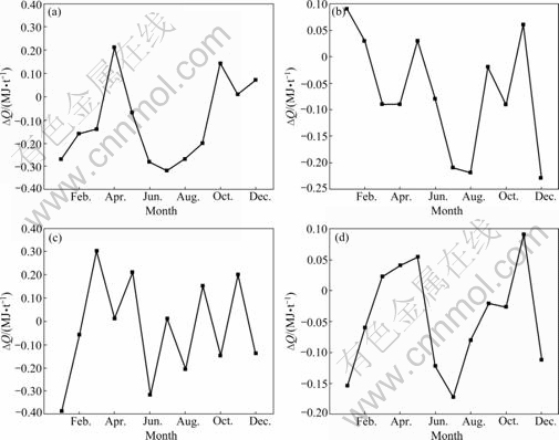
Fig.1 Forecasting absolute errors of energy consumption in copper refining process: (a) Model in Ref.[11]; (b) Model in Ref.[12];  (c) Model in Ref.[15]; (d) Proposed new nonlinear combined forecasting model

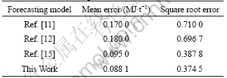
It is very obvious in Fig.1 and Table 3 that the forecasting results from the new nonlinear combined forecasting model based on fuzzy adaptive variable weight is of higher precision compared with other single forecasting models.

3 Application of new nonlinear combined forecasting model

3.1 Fuzzy adaptive variable weight combined forecasting of oxygen consumption

Because the quality and output of nonferrous metal smelting directly depend upon the consumption of oxygen, the new nonlinear fuzzy adaptive variable weight combined forecasting model was used to predict the oxygen consumption of a heavy nonferrous metal smelter. The results are shown in Table 4.

Table 4 Oxygen consumption data and their relative errors

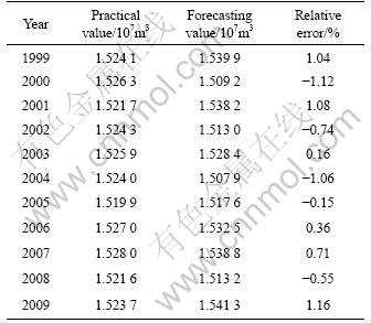
Based on oxygen consumption data from 1999 to 2007 shown in Table 4, the oxygen consumption of the year 2008 and 2009 was predicted by using the method of fuzzy adaptive variable weight, and some forecasting values and errors about the oxygen consumption were obtained. Compared with those of test data, the forecasting relative errors of oxygen consumption in the nonferrous metals smelter are -0.55% and 1.16%, respectively. Therefore, the new nonlinear combined forecasting model based on fuzzy adaptive variable weight is of higher accuracy.

3.2 Fuzzy adaptive variable weight combined forecasting and management system for enterprise energy consumption

The forecasting of energy consumption of an enterprise must be based on abundant inter-related historical data, and a large amount of added-weight calculation has to be done for the forecasting model due to numerous variables involved. With Visual Basic 6.0 as a platform, a fuzzy adaptive variable weight combined forecasting and management system was developed, which can not only facilitate calculation, but also raises accuracy.

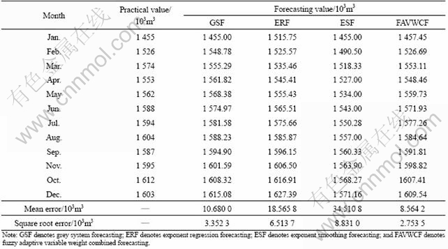
In this example, firstly, gas consumption statistical data of 12 months in 2009 were assigned to each subsystem, then grey forecasting, exponential regression forecasting and exponential smoothing forecasting on the statistical data were worked out. The forecasting results are shown in Table 5. Then, fuzzy adaptive variable weight combined forecasting on the basis of the above three single forecasting results was done. The forecasting results are shown in the last column of Table 5. A convenient Visual Basic 6.0 forecasting process was accomplished.

The mean error of the above adaptive variable weight combined forecasting method is 8.564 2×10³ m³, and the square-root error is 2.753 5×10³ m³. Evidently, even when regular models such as grey forecasting model, exponent regression forecasting model and exponential smoothing forecasting model are used, after their forecasting results are combined by using the fuzzy adaptive variable weight combined forecasting method, the forecasting accuracy will be increased and forecasting result will be better.

Therefore, with the fuzzy adaptive variable weight combined forecasting and management system based on Visual Basic 6.0 platform, the time and amount of calculation of combined forecasting will be greatly reduced, and the accuracy will be substantially increased. The system provides a powerful calculation tool for the forecast of energy consumption of enterprises.

4 Conclusions

(1) A new nonlinear combined forecasting model is established by using the conceptions such as the relative error, the change tendency of the forecasted object, gray basic weight and adaptive control coefficient based on the method of fuzzy variable weight. The results reveal that mean errors and square root errors of forecasting values from the new nonlinear combined forecasting model are smaller than those of other combined forecasting model, that is to say, the forecasting precision from the new nonlinear combined forecasting model is higher than that of other combined forecasting models.

Table 5 Practical and forecasting values of fuzzy adaptive variable weight combined forecasting and management system

 (2) The combined forecasting model is suitable for nonlinear time series in some complex industry system with a small quantity of data. It is very useful for requirements and the decision in complex industry system. A new forecasting idea for enhancing forecasting precision can be gotten from the combined forecasting model.

(3) The forecasting accuracy of some regular forecasting models is lower. Once their forecasting results are combined by using the fuzzy adaptive variable weight combined forecasting method, new forecasting results with higher accuracy will be obtained.

References

[1] BARRY F, ANINDYA R. Forecasting using the trend model with autoregressive errors [J]. International Journal of Forecasting, 2005, 21(2): 291-302.

[2] YUAN Fang-ming, WANG Xing-hua, ZHANG Jiong-ming, ZHANG Li. Online forecasting model of tundish nozzle clogging [J]. Journal of University of Science and Technology Beijing: Mineral, Metallurgy, Material, 2006, 13(1): 21-24.

[3] MICHAEL S L B, TIEN C. Forecasting presidential elections: When to change the model [J]. International Journal of Forecasting, 2008, 24(2): 227-236.

[4] WU Xiao-ling, WANG Chuan-hai, CHEN Xi, XIANG Xiao-hua, ZHOU Quan. Kalman filtering correction in real-time forecasting with hydrodynamic model [J]. Journal of Hydrodynamics, 2008, 20(3): 391-397.

[5] MOHAMMADI K, ESLAMI H R, KAHAWITA R. Parameter estimation of an ARMA model for river flow forecasting using goal programming [J]. Journal of Hydrology, 2006, 331(1/2): 293-299.

[6] CHENG C H, CHEN Y S, WU Y L. Forecasting innovation diffusion of products using trend-weighted fuzzy time-series model [J]. Expert Systems with Applications, 2009, 36(2): 1826-1832.

[7] AGAMI N, ATIYA A, SALEH M, EL-SHISHINY H. A neural network based dynamic forecasting model for trend impact analysis [J]. Technological Forecasting and Social Change, 2009, 76(7): 952-962.

[8] KOMORN?K J, KOMORN?KOV? M, MESIAR R, SZ?KEOV? D, SZOLGAY J. Comparison of forecasting performance of nonlinear models of hydrological time series [J]. Physics and Chemistry of the Earth: Parts A/B/C, 2006, 31(18): 1127-1145.

[9] L?F M, LYHAGEN J. Forecasting performance of seasonal cointegration models [J]. International Journal of Forecasting, 2002, 18(1): 31-44.

[10] TSEKOURAS G J, DIALYNAS E N, HATZIARGYRIOU N D, KAVATZA S. A non-linear multivariable regression model for midterm energy forecasting of power systems [J]. Electric Power Systems Research, 2007, 77(12): 1560-1568.

[11] TSAUR R C. The development of an interval grey regression model for limited time series forecasting [J]. Expert Systems with Applications, 2010, 37(2): 1200-1206.

[12] LI Xue-quan, LI Chun-sheng. An improved method of fuzzy variable weight combination forecasting [J]. Journal of Central South University of Technology: natural Science, 2003, 34(6): 708-710. (in Chinese)

[13] BAR-GERA H, BOYCE D. Solving a non-convex combined travel forecasting model by the method of successive averages with constant step sizes [J]. Transportation Research Part B: Methodological, 2006, 40(5): 351-367.

[14] ZOU Hui, YANG Yu-hong. Combining time series models for forecasting [J]. International Journal of Forecasting, 2004, 20(1): 69-84.

[15] TANG X W, ZHOU Z F, SHI Y. The variable weighted functions of combined forecasting [J]. Computers and Mathematics with Application, 2003, 45(4/5): 723-730.

Foundation item: Project(08SK1002) supported by the Major Project of Science and Technology Department of Hunan Province, China

Received date: 2010-01-03; Accepted date: 2010-03-19

Corresponding author: JIANG Ai-hua, Doctoral candidate; Tel: +86-731-85628323; E-mail: jah65@163.com

(Edited by CHEN Wei-ping)