
J. Cent. South Univ. (2016) 23: 817-824
DOI: 10.1007/s11771-016-3128-7

Comparison of three formulations for eddy-current problems in a spiral coil electromagnetic acoustic transducer
SHI Wen-ze(ʯ����)1, 2, WU Yun-xin(������)1, 2, 3, GONG Hai(����)1, 2, 3, 4,
ZHAO Zhi-ran(��־Ȼ)1, 2, FAN Ji-zhi(����־)1, 3, TAN Liang-chen(̷����)1, 2
1. State Key Laboratory of High Performance Complex Manufacturing (Central South University),
Changsha 410083, China;
2. School of Mechanical and Electrical Engineering, Central South University, Changsha 410083, China;
3. Nonferrous Metal Oriented Advanced Structural Materials and Manufacturing Cooperative Innovation Center, Changsha 410083, China;
4. School of Materials Science and Engineering, Central South University, Changsha 410083, China
 Central South University Press and Springer-Verlag Berlin Heidelberg 2016
Abstract:
Three differential equations based on different definitions of current density are compared. Formulation �� is based on an incomplete equation for total current density (TCD). Formulations �� and �� are based on incomplete and complete equations for source current density (SCD), respectively. Using the weak form of finite element method (FEM), three formulations were applied in a spiral coil electromagnetic acoustic transducer (EMAT) example to solve magnetic vector potential (MVP). The input impedances calculated by Formulation III are in excellent agreement with the experimental measurements. Results show that the errors for Formulations I & II vary with coil diameter, coil spacing, lift-off distance and external excitation frequency, for the existence of eddy-current and skin & proximity effects. And the current distribution across the coil conductor also follows the same trend. It is better to choose Formulation I instead of Formulation III to solve MVP when the coil diameter is less than twice the skin depth for Formulation I is a low cost and high efficiency calculation method.
Key words:
1 Introduction
Electromagnetic acoustic transducers (EMATs) have been an important ultrasonic non-destructive evaluation (NDE) technique for electrically conducting materials. It can be rapidly scanned across a sample as there is no acoustic coupling medium, which is especially desirable in on-line or hostile environmental measurement conditions. This is usually due to the sample being hot, moving, or otherwise not suitable for a transducer to be placed on it directly, or when no coupling media or surface preparations are permissible [1-4]. EMAT has advantages in non-contact operation, high-efficiency inspection, long-rang inspection, high temperature operation and different types of ultrasonic waves [5-9].
For noferromagnetic material, EMATs are able to generate and detect ultrasonic waves mainly because of the Lorentz force phenomenon. The Lorentz force arises in any electrically conducting material because of an interaction between the static magnetic flux and the pulse eddy current, and concentrated into a skin depth at the surface of the material [10].
Skin and proximity effects are two important electromagnetic effects in the modeling of EMAT, which are significantly obvious in high-frequency case when two current-carrying conductors are very close. Electromagnetic skin effect is the tendency of an alternating current imposed on a conductor to pull to the surface of the conductor. Proximity effect, defined as how the magnetic field generated by current flowing in one conductor, affects the current distribution in a neighboring conductor.
Most of researchers tend to use Formulations II and III to solve pulsed eddy current in the EMAT modeling, but seldom of them choose Formulation I [11-16]. In Refs. [15-16], Formulation I is used in the modeling of a meander coil EMAT. In Refs. [11-12], Formulation II is used to the spiral coil EMATs. In Ref. [11], the proximity and skin effects are neglected for small coil dimensions, small coil dimensions, relatively large coil spacing and low excitation frequency. In Ref. [13], using Galerkin��s criterion to Formulation III, an FEM to solve steady-state skin effects problems is presented. In Ref. [14], the FEM results from Formulations II & III are compared at two different frequencies: 0.5 MHz and 2 MHz. The effects of lift-off distance and coil spacing on the Lorentz force calculated from Formulation III are also investigated. They indicate that if proximity and skin effects are ignored, the error for Formulation II will increase to 75% for rectangular conductors with 0.10 mm height and 0.50 mm width. In Refs. [15-16], a 2-D configuration of a mender coil EMAT is modeled to compare the results from Formulations I, II and III. The Lorentz forces from the three formulations are investigated in four cases, in which only coil height and excitation frequency are changed. It is concluded that the error for Formulation I is less than Formulation II.
Skin and proximity effects are considered in Formulation III. However, Formulations I and II do not take into account these effects. For Formulation III, finite elements around the coil conductor borders should be refined sufficiently in order to get a more accurate result, and also a smaller calculation time step is needed. It requires a higher performance computer and takes a longer time for the calculation. For Formulation I, no such refinement is needed. A larger calculation time step can be used in Formulation I to get a consistent result, compared to Formulation III. So, Formulation I computes faster and has lower requirements for computers. The calculation speed of Formulations II is slower than Formulation I, but faster than Formulation III. In other words, Formulation III is a time-consuming method compared to Formulation I, but it can get a more accurate results. However, the conditions for the replacement of Formulation III with Formulation I have not been given in the published works.
In this work, 2-D axisymmetric structure of EMAT models consisting of six conductors above an aluminum specimen is modeled by using Formulations I, II and III. The verification experiments are accomplished to validate the validity and accuracy of the input impedances calculated by Formulation III. Varying the coil diameters, its spacing, lift-off distances and excitation frequencies, the induced current densities from three formulations are compared. Upon on these results, the errors for Formulations I and II are compared. The effects of such parameters on the eddy-current, skin and proximity effects are also investigated. The conditions for the replacement of Formulation III with Formulation I are also studied in the modeling of the spiral coil EMATs.
2 Magnetic field equation
For a 2-D axisymmetric multi current-carrying conductor analysis, the magnetic field is obtained in terms of the magnetic vector potential (MVP) in the region of solution from the following equations:
 (1)
(1)
 (2)
(2)
 (3)
(3)
where �� and �� are the permeability and conductivity, respectively; A��, J��k, Jsk, ik(t) and Rk denote MVP, total current density (TCD), source current density (SCD), total current and cross-sectional region of the k-th conductor, respectively.
In source-free conducting region, Jsk is assumed to be 0, the MVP must satisfy:
 (4)
(4)
1) Formulation I.
In this formulation, the TCD is assumed to be known and independent of position inside an conductor. Thus, a incomplete equation for TCD J��k is given as [15-16]
 (5)
(5)
 (6)
(6)
where ak represents the area of the k-th conductor. Combining Eqs. (5), (6) and (1), the differential equation inside the exciting coil conductor can be expressed as
 (7)
(7)
2) Formulation II.
In this equation, Jsk is assumed to be the only function of total current. Usually, an incomplete equation for SCD Jsk can be given as follows [14-16]
 (8)
(8)
Combining Eqs. (8), (1) and (2), the differential equation inside the exciting coil conductor can be written as
 (9)
(9)
3) Formulation III.
Adding a single integrodifferential equation to the incomplete equation for SCD, a complete equation for SCD Jsk can be obtained as [14-16]
 (10)
(10)
Combining Eqs. (10), (1) and (2), the differential equation inside the exciting coil conductor becomes
 (11)
(11)
In Eqs. (7), (9) and (11), if the differential operator  /t is replaced with j��, the harmonic formulations can be used to solve MVP in frequency domain. The resistance Rk and inductance Lk of the k-th conductor can be given as [17]
 (12)
(12)
 (13)
(13)
 (14)
(14)
where Ik is the effective value of ik; Hk is the magnetic field intensity of Hk.
When time-varying current is passing through a coil above a sample surface, the electromagnetic waves emitted from the coil will induce an eddy current in the sample within the skin-depth ��, which is defined by the depth at which the current density is attenuated by 1 Napier (in the ratio 1/e=1/2.72), given by
 (15)
(15)
where �� denotes as the external excitation angular frequency.
3 Method
Figure 1 shows the 2-D axisymmetric configuration of the bulk wave EMAT. A permanent magnetic is used to provide static magnetic field perpendicular to the spiral coil and specimen placed bellow. The coil is placed above the specimen. When the coil is provided by the pulse excitation current with the desired frequency, the ultrasonic wave can be generated by Lorentz force and propagates perpendicularly to the surface of aluminum specimen. The spiral coil can be viewed as arrays of N concentric conductor circles. N refer to turns of the coil. a and b are the radius and height of the permanentmagnet, respectively. c refers to the distance between the magnet and coil. d, s, r0 and h denote the coil conductor diameter, coil spacing, coil inner radius and lift-off distance, respectively.
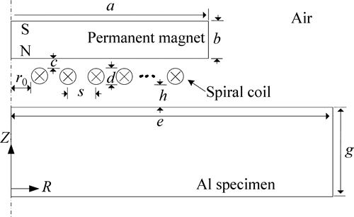
Fig. 1 Configuration of bulk wave EMAT, spiral coil, magnet and specimen
In order to solve MVP based on Formulations I, II and III, the weak form of partial differential equation (PDE) in the finite element software COMSOL Multiphysics was used. This built-in mathematical interface only needs to specify a PDE and its boundary conditions on weak form.
The weak form of Formulation �� is obtained as

 (16)
(16)
where /n denotes the differentiation in the outward normal direction to the boundary surface.
The weak form of Formulation II is obtained as


 (17)
(17)
The weak form of Formulation �� is obtained as


 (18)
(18)
In Eqs. (16), (17) and (18), when the differential operator /t is replaced with j��, the modified weak form formulations can be used to solve MVP in frequency domain.
In order to correctly resolve the eddy current density around the surface of the aluminum specimen and the current distribution in the cross-sectional region of coil conductors, more than nine meshes across 3 times the skin depth should be made. The mesh elements and the time steps should be adjusted for a more accurate calculation.
The transient exciting current of the k-th conductor is given as [14]
 (19)
(19)
where I0 is a constant value; ��0=2��f0 is the angular centre frequency; n is the number of cycles.
The prosperities of the specimen are: conductivity ��AL=3.571��107 S/m, permeability ��AL=1. The spiral coil is made of copper with conductivity ��Cu=2.667��107 S/m, permeability ��Cu=1. The prosperities of the permanent magnet are: conductivity ��FM=7.143��105 S/m, permeability ��PM=1.04. Here, I0=30 A, n=2, a=18.8 mm, b=8.2 mm, c=0.2 mm, r0=1 mm, e=20 mm, g=10 mm, N=20 were chosen.
4 Experimental validation
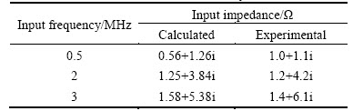
For validating the results calculated by Formulation ��, input impedances of three tightly-wounded coils at 1 MHz frequency were measured by an impedance analyzer HP 8714C. Also, input impedances of the coil with diameter 0.5 mm in 19 turns were measured at frequencies 0.5 MHz, 2 MHz and 3 MHz. Results listed in Tables 1 and 2 show that the calculated resultsand measured ones are in good agreement, which validates the validity and accuracy of the results from Formulation III.
Table 1 Input impedances by calculation (from Formulation ��) and measurement from three different diameters (��0.25 mm, ��0.35 mm, ��0.5 mm) coils with same outer diameter in existence of permanent magnet and aluminum specimen at 1 MHz, c=0.2 mm, h=0.2 mm, r0=1 mm.
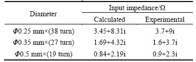
Table 2 Input impedances by calculation (from Formulation III) and measurement from a coil (��0.5 mm��19 turns) in existence of permanent magnet and aluminum specimen at frequencies 0.5, 2, and 3 MHz, c=0.2 mm, h=0.2 mm, r0=1 mm
5 Results and discussion
A spiral coil EMAT transmitter is modeled in time domain by varying input frequency, coil diameter, lift-off distance and coil spacing. The effects of all the above variables on the induced current density (ICD) (underneath the tenth source conductor from the right, at the skin depth surface of the aluminum specimen) from the three formulations will be investigated. The absolute maximum value of the induced current density in time domain is used as an indicator for such effects.
If Formulation III is regarded as the exact value, the relative errors for Formulations I and II can be defined as
 (20a)
(20a)
 (20b)
(20b)
where II, III and IIII are the absolute maximum values of induced current density in time domain from Formulations I, II and III, respectively.
In order to reflect the inhomogeneity of the current distribution in the conductor cross-sectional region, a parameter Q is introduced. It is defined by
 (21)
(21)
 (22)
(22)
where R and J��,max are the conductor cross-sectional area and the absolute maximum value of the current density in the conductor area R, respectively, e is equal to 2.72. The larger the Q is, the more inhomogeneous the current density in conductor cross-area will be.
Figure 2 shows that the induced current densities from Formulations I, II and III decrease when the coil diameters increase. This is because the current density is reduced when enlarging coil diameters with fixed total current. The errors for Formulations I and II increase with the coil diameter. The error for Formulation I is approximately 0 when coil diameters are less than 0.2 mm, but for 0.5 mm, it increases to 5.9%. When the coil diameter is 0.02 mm, the error for Formulation II is 20.5%, but for 0.5 mm, it reaches 98.8%.
Figure 3 shows the effect of varying the coil diameter d on the normalized current density across the tenth conductor from the left in frequency domain in two cases: (a) d=0.5 mm; (b) d=0.2 mm. Figures 3(a) and (b) depict that the current densities are high close to theborders and decrease rapidly inside the conductors. That means that the smaller the coil diameter is, the greater the Q is, and the more inhomogeneous the current distribution is. The errors for Formulations I and II will be larger if the current distribution in the coil cross-section area is more inhomogeneous. When the ratio d/�ġ�2 (for aluminum at 1 MHz, ��=0.11 mm), Formulation I can be used to solve MVP instead of Formulation III. When the coil diameter is about 20% of ��, there is still an error of 20.5% for Formulation II.
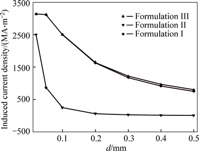
Fig. 2 Comparison of FEM results from Formulations I, II and III when adjusting coil diameter d at 1 MHz, s=0, h=0.5 mm

Fig. 3 Current density (normalized) from Formulation III when varying coil dimensions in frequency domain at 1 MHz, s=0, h=1 mm:
Figure 4 shows that the induced current densities from the three formulations decrease when the conductors spacing is increased. The errors for Formulations I and II also follow the same trend. When the coil spacing is 0.02 mm, the error for Formulation I is 5.2%, while the error for Formulation II is 98.8%. When the coil spacing is 0.4 mm, the error for Formulation I is 2.0%, while the error for Formulation II is 98.1%. Compared with the error for Formulation II, the error for Formulation I is more sensitive to the coil spacing. It is likely that when the ratio s/d��1, Formulation I can be used to solve MVP instead of Formulation III.
Figure 5 shows the effect of varying the coil spacing s on the normalized current density across the tenth conductor from the left in frequency domain in fourcases: (a) N=1; (b) s=0.1 mm, N=20; (c) s=0.3 mm, N=20; (d) s=0.4 mm, N=20. Figure 5(a) depicts a single conductor without any one adjacent to it, so only skin effect is considered. For two adjacent conductors each carrying the same direction alternating currents, the external magnetic fields of the two conductors will attract each other. Figures 5(b)-(d) show that the less the coil spacing is, the more the current density will move away from the adjacent borders of the conductors. As shown in Fig. 6, due to the eddy-current effect existing in the magnet and specimen, the current densities Jup and Jdown will shift to the coil conductor borders which are near to the magnet and specimen. And because of theproximity effect existing in the conductors, the current densities Jlefl and Jright will move away from the adjacent borders of the conductors. So, the less the coil spacing is, the more the current density will move away from the adjacent borders of the conductors to ones which are near to the magnet and specimen. The Q value will increase with the coil spacing. That means that the less is the coil spacing, the more obvious the proximity effect is. Because more of the current distribution is moving to the borders near to the magnet and specimen, the induced current in the material will be larger.
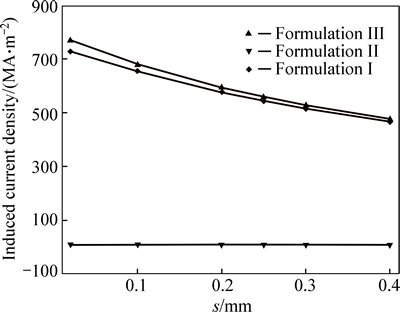
Fig. 4 Comparison of FEM results from Formulations I, II and III when adjusting coil spacing s at 1 MHz, d=0.5 mm, h=0.5 mm
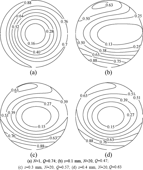
Fig. 5 Current density (normalized) from Formulation III in frequency domain when varying the coil spacing at 1 MHz, d=0.5 mm, h=0.5 mm:
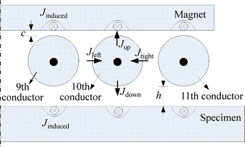
Fig. 6 Current density distribution trends of conductors considering proximity and eddy-current effects
Figure 7 shows the effect of varying the lift-off distance on the induced current. The closer the coil to the material is, the stronger the induced current in it will be. When the coil diameter is 0.5 mm and the lift-off is reduced from 1.5 mm to 0.1 mm, the induced current from Formulation III will reach 37.7%. When the diameter is varied from 0.3 mm to 0.1 mm, those forces will range from 66.6% to 306.7%. So, the lift-off is important to the accuracy of the EMAT measurement. For those EMATs used in the scanning of rough surface forgings or special cases in which the lift-off can��t be kept constant, a larger diameter coil will be a good choice. Figure 7(b) shows that the error for Formulation I increases when the lift-off is reduced. But the error for Formulation II has the reverse trend. The error for Formulation II is larger than one for Formulation I. The larger the coil diameter is, the greater the errors for Formulations I and II will be. When the ratio h/d��3, the error for Formulation I is no more than 2%.
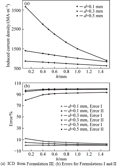
Fig. 7 Comparison of FEM results from Formulations I, II and III when adjusting lift-off h at 1 MHz, s=0:
Figure 8 shows the effect of varying the lift-off h on the normalized current density across the tenth conductor from the left in frequency domain in four cases: (a) h= 0.1 mm; (b) h=0.6 mm; (c) h=1.0 mm; (d) h=1.5 mm. Due to the eddy-current effect, when the lift-off increases, the current density Jdown (shown in Fig. 6) will decrease, while the current density Jup will increase. The current density will move away from the borders which are near the specimen to ones that are near the magnet. When the lift-off reduces from 1.5 mm to 0.1 mm, the Q will increase first and then decrease. So, in order to enhance the current density Jdown, the magnet-to-coil distance should not be too small.
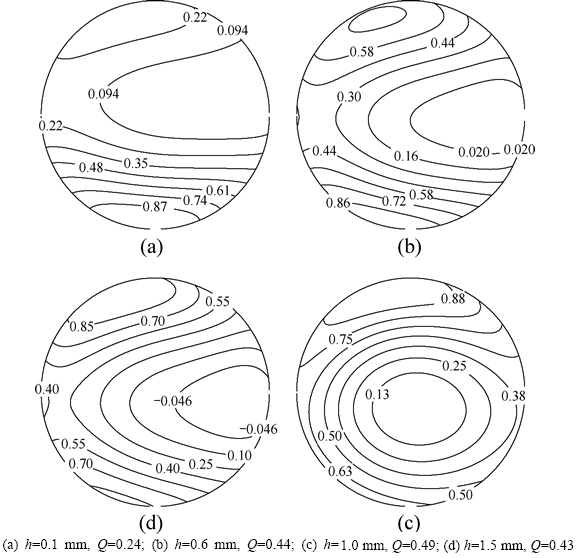
Fig. 8 Current density (normalized) from Formulation III in frequency domain when varying lift-off at 1 MHz, s=0, d=0.5 mm:
Figure 9 shows the effect of the induced current in the marital by varying the external excitation frequency. The induced current in the skin depth of the specimen increases with the frequency. And the errors for Formulations I and II follow the same trend. When the frequency is 0.05 MHz, the error for Formulation I is 0.2%, and for Formulation II is 66.7%. When the frequency is 2.5 MHz, the error for Formulation I is 7.2%, and for Formulation II is 98.3%. When the frequency is no more than 0.2 MHz (in this case, d/�ġ�2), the error for Formulation I is less than 2%.
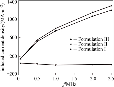
Fig. 9 Comparison of FEM results from Formulations I, II and III when adjusting external excitation frequency at d=0.5 mm, s=0, h=0.5 mm
Figure 10 shows the effect of varying external excitation frequency on the normalized current distribution across the tenth conductor from the left in frequency domain in two cases: (a) f=0.5 MHz, (b) f= 2.5 MHz. The Q of 2.5 MHz is smaller than that of 0.5 MHz. When the frequency is increased, most of the current is distributed in a smaller skin depth, making the skin effect more obvious. Due to the current density moving to the conductor borders, the induced current will increase. The more inhomogeneous current distribution will contribute to greater errors for Formulations I and II.
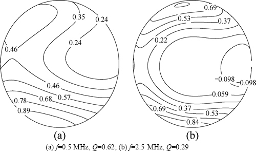
Fig. 10 Current density (normalized) from Formulation III in frequency domain when varying external excitation frequency at s=0, d=0.5 mm, h=0.5 mm:
6 Conclusions
1) Formulations I ignores the dependence of total current density on position, so the degree of uniformity in current distribution determines the errors for Formulations I. In the spiral coil EMAT modeling, when the coil diameter is less than twice the skin depth, Formulation I can be used to solve MVP instead of Formulation III, with an error of no more than 2%.
2) Compared to Formulation III, Formulation II ignores the integral form of Maxwell��s second equation, so the skin and proximity effects are neglected. The error for Formulation II increases with both source conductor dimensions and the time derivative of the MVP. It is more sensitive to the coil diameter and external excitation frequency than to the coil spacing and the lift-off. It seems that Formulation II is hard to get a consistent result with Formulation III when the coil diameter or the frequency is not small enough. When the coil diameter is less than 20% of the skin depth or the frequency is less than 0.05 MHz, there is still an error of more than 20% in Formulation II.
3) Coil diameter, coil spacing, and excitation frequency determine the eddy-current, skin and proximity effects in the EMAT modeling. In order to improve the induced current in a specimen, the magnet-to-coil distance should not be too small, and the coil spacing should not be too large.
References
[1] HERNANDEZ-VALLE F, DIXON S. Initial tests for designing a high temperature EMAT with pulsed electromagnet [J]. NDT & E International, 2010, 43(2): 171-175.
[2] PETCHER P A, POTTER M D G, DIXON S. A new electromagnetic acoustic transducer (EMAT) design for operation on rail [J]. NDT & E International, 2014, 65: 1-7.
[3] JIAN X, DIXON S, EDWARDS R, QUIRK K, BAILLIE I. Effect on ultrasonic generation of a backplate in electromagnetic acoustic transducers [J]. Journal of Applied Physics, 2007, 102(2): 249091-249096.
[4] HAO Kuan-sheng, HUANG Song-hing, ZHAO Wei, DUAN Ru-jiao, WANG Shen. Modeling and finite element analysis of transduction process of electromagnetic acoustic transducers for nonferromagnetic metal material testing [J]. Journal of Central South University of Technology, 2011, 18: 749-754.
[5] HIRAO M, OGI H. EMATs for science and industry: Noncontacting ultrasonic measurements [M]. New York: Springer, 2003.
[6] ZHAI Guo-fu, WANG Kai-can, WANG Ya-kun, KANG Lei. Modeling of Lorentz forces and radiated wave fields for bulk wave electromagnetic acoustic transducers [J]. Journal of Applied Physics, 2013, 114(5): 549011-549019.
[7] KANG L, DIXON S, WANG K C, DAI J M. Enhancement of signal amplitude of surface wave EMATs based on 3-D simulation analysis and orthogonal test method [J]. NDT & E International, 2013, 59: 11-17.
[8] DING X, WU X, WANG Y. Bolt axial stress measurement based on a mode-converted ultrasound method using an electromagnetic acoustic transducer [J]. Ultrasonics, 2014, 54(3): 914-920.
[9] TU J, KANG Y, LIU Y. A new magnetic configuration for a fast electromagnetic acoustic transducer applied to online steel pipe wall thickness measurements [J]. Materials Evaluation, 2014, 72(11): 1407-1413.
[10] RIBICHINI R, CEGLA F, NAGY P B, CAWLEY P. Quantitative modeling of the transduction of electromagnetic acoustic transducers operating on ferromagnetic media [J]. Ultrasonics, Ferroelectrics, and Frequency Control, IEEE Transactions on, 2010, 57(12): 2808-2817.
[11] HAO K, HUANG S, ZHAO W, WANG S, DONG J R. Analytical modelling and calculation of pulsed magnetic field and input impedance for EMATs with planar spiral coils [J]. NDT & E International, 2011, 44(3): 274-280.
[12] JIAN X, DIXON S, GRATTAN K, EDWARDS R S. A model for pulsed Rayleigh wave and optimal EMAT design [J]. Sensors and Actuators A: Physical, 2006, 128(2): 296-304.
[13] KONRAD A. Integrodifferential finite element formulation of two- dimensional steady-state skin effect problems [J]. Magnetics, IEEE Transactions on, 1982, 18(1): 284-292.
[14] JAFARI-SHAPOORABADI R, KONRAD A, SINCLAIR A N. Improved finite element method for EMAT analysis and design [J]. Magnetics, IEEE Transactions on, 2001, 37(4): 2821-2823.
[15] JAFARI-SHAPOORABADI R, KONRAD A, SINCLAIR A N. Comparison of three formulations for eddy-current and skin effect problems [J]. Magnetics, IEEE Transactions on, 2002, 38(2): 617-620.
[16] JAFARI SHAPOORABADI R. Electromagnetic acoustic transducer analysis by the finite element method [D]. Toronto: University of Toronto (Canada), 2002.
[17] HAO Kuan-Sheng, HUANG Song-Ling, ZHAO Wei, WANG Shen. Circuit-field coupled finite element analysis method for an electromagnetic acoustic transducer under pulsed voltage excitation [J]. Chinese Physics B, 2011, 20(6): 681041-681048.
(Edited by DENG L��-xiang)
Foundation item: Project(2014BAF12B01) supported by the Key Projects in the National Science & Technology Pillar Program during the Twelfth Five-year Plan Period, China; Project(51405520) supported by the National Natural Science Foundation of China; Project(2012CB619505) supported by National Basic Research Program of China
Received date: 2015-01-11; Accepted date: 2015-06-15
Corresponding author: GONG Hai, Lecturer; Tel: +86-731-88660476; E-mail:gonghai@csu.edu.cn
Abstract: Three differential equations based on different definitions of current density are compared. Formulation �� is based on an incomplete equation for total current density (TCD). Formulations �� and �� are based on incomplete and complete equations for source current density (SCD), respectively. Using the weak form of finite element method (FEM), three formulations were applied in a spiral coil electromagnetic acoustic transducer (EMAT) example to solve magnetic vector potential (MVP). The input impedances calculated by Formulation III are in excellent agreement with the experimental measurements. Results show that the errors for Formulations I & II vary with coil diameter, coil spacing, lift-off distance and external excitation frequency, for the existence of eddy-current and skin & proximity effects. And the current distribution across the coil conductor also follows the same trend. It is better to choose Formulation I instead of Formulation III to solve MVP when the coil diameter is less than twice the skin depth for Formulation I is a low cost and high efficiency calculation method.
