
J. Cent. South Univ. Technol. (2010) 17: 587-592
DOI: 10.1007/s11771-010-0527-z ![]()
3-D direct current resistivity forward modeling by
adaptive multigrid finite element method
TANG Jing-tian(������)1, WANG Fei-yan(������)1, REN Zheng-yong(������)1, 2, GUO Rong-wen(������)1, 3
1. School of Info-physics and Geomatics Engineering, Central South University, Changsha 410083, China;
2. Institute of Geophysics, ETH Zurich-Swiss Federal Institute of Technology, Zurich 8093, Switzerland;
3. School of Earth and Ocean Sciences, University of Victoria, Victoria 1700, Canada
? Central South University Press and Springer-Verlag Berlin Heidelberg 2010
Abstract:
Based on the fact that 3-D model discretization by artificial could not always be successfully implemented especially for large-scaled problems when high accuracy and efficiency were required, a new adaptive multigrid finite element method was proposed. In this algorithm, a-posteriori error estimator was employed to generate adaptively refined mesh on a given initial mesh. On these iterative meshes, V-cycle based multigrid method was adopted to fast solve each linear equation with each initial iterative term interpolated from last mesh. With this error estimator, the unknowns were nearly optimally distributed on the final mesh which guaranteed the accuracy. The numerical results show that the multigrid solver is faster and more stable compared with ICCG solver. Meanwhile, the numerical results obtained from the final model discretization approximate the analytical solutions with maximal relative errors less than 1%, which remarkably validates this algorithm.
Key words:
adaptive multigrid; a-posteriori error estimator; unstructured mesh; V-cycle; finite element method��
1 Introduction
In electromagnetic computations, finite element method [1-4] which owns reliable mathematical theories and the capability of dealing with complex geological models is the most outstanding one in all numerical methods. In the finite element method the conventional way for mesh generation was according to the operators�� experiences and some priori information [5] by which satisfactory results were usually obtained. As it was well known that the complicated distribution of electric field in direct current (DC) resistivity modeling requested the distribution of the unknowns to be as reasonable as possible. When problems became complex, accuracy requirement could not always be met by artificial work. Moreover, numerical results calculated from standard finite element method were determined from just once mesh generation, which meant that the accuracy would be controlled partly by the operators�� experiences. Finally, as the required models became complicated and large- scaled, which resulted in large amount of nodes being created, commonly used solvers in DC resistivity modeling like traditional CG-type ones might not work so efficiently.
Aiming at avoiding artificial model discretization,much attention was paid to finite element method combined with certain error estimator(s), which is usually called adaptive finite element method (AFEM). According to our knowledge, the adaptive technique has been widely used for a class of problems [6-7]. In electromagnetic computations, its applications in 2-D magnetotelluric [8] and 2-D marine controlled-source problem [9] were respectively implemented. STEPHAN et al [10] presented an hp-version of the finite element/ boundary element coupling method to solve eddy current problem for the time-harmonic Maxwell equations. Moreover, analysis about application of adaptive finite element method in geo-electromagnetic field was also discussed [11]. Although the adaptive procedure has shown good performances, its application in DC field is still in the preliminary stage.
Moreover, to guarantee the efficiency and accuracy when solving the resulting linear equation system derived form the finite element computations, multigrid algorithm [12-14] which exhibited optimal computational performance was mostly focused. Inspired by the efficiency and reasonability of error estimators and multigrid method, a new adaptive multigrid finite element method was presented in this work. On a given initial mesh, the a-posteriori error estimator based on gradient recovery technique was employed to evaluate the rationality of current model discretization and thenpredict a new reasonable one. In the whole process, several iterative meshes were generated, on each of which V-cycle based multigrid solver [12] was adopted to solve the linear equation. In terms of linear time complexity of multigrid algorithm, each large linear equation could be fast solved. After this adaptive process was terminated, approximately accurate results could be obtained from the final locally refined mesh.
2 Theory basis
2.1 Finite element method
Generally, the boundary value problem of DC resistivity forward modeling can be described as follows:
 (1)
(1)
where u is the unknown electric potential, �� is the conductivity in the specific domain, I(=1 A) is the current, x is a potential point, xA is the position of the current source point, �� is the solution domain, ��N is the air-earth interface where the Neumann boundary condition is taken, ��M is the outer boundary of �� at which ?��=��N+��M is satisfied, n is the outer unit normal vector, �� is the Delta function, r is the distance from current source point xA to potential point x on ��M, and �� is the angle between the outward normal n and vector r=x-xA.
With operations like integral by parts and Green integral, the integral week form [17] of Eq.(1) was reduced to
![]()
![]() (2)
(2)
where w is a testing function in the same space with u. In finite element process, u is approximated by a summation of unknown value ui and shape function Ni at
each node i like ![]() By substituting this formula
By substituting this formula
into Eq.(2), the Galerkin-weighted residual expression [17] was obtained with the testing function being specified as the shape function
![]()
![]() (3)
(3)
where n is the total number of nodes. In the form of matrix symbol, the above formula could be re-written as:
 (4)
(4)
Each single term in Eq.(4) was obtained by an assembly after looping on each element. Here, linear unstructured tetrahedron was adopted due to its flexibility of fitting complicated boundaries. Given a tetrahedron element![]() with four vertices vi (i=0, 1, 2, 3), its contribution to the volume integral of K could be described as:
with four vertices vi (i=0, 1, 2, 3), its contribution to the volume integral of K could be described as:
![]() (5)
(5)
where V is the volume of ��, the coefficients ajai, bjbi and cjci are simply associated with the coordinates of vertices vi [18]. If a triangular face �� of �� was on boundary ��M, the face integral part of K in �� could be written as:
 (6)
(6)
where S is the area of ��. Here, it should be noted that this face integral term is not related with vi on �� but only with triangle��s area. As for the right hand side F, it has a value of I only at the current source point xA and of zero at other else place, which could be easily deduced by the property of �� function.
2.2 Adaptive multigrid algorithm
As for linear equations, the residual r=KU-F usually owns two components which are respectively denoted by high-frequency component and low- frequency component [12]. Usually, oscillatory modes (also called high-component) of the error are eliminated effectively, by contrast, smooth (low-component) modes damp very slowly in iterative methods. To fix this problem, two principal techniques were employed in multigrid method, which were respectively relaxation and coarse-grid correction. Generally, two steps are needed to implement the multigrid algorithm. In the first step, a sequence of restriction (mapping from fine grid to coarse grid), prolongation (from coarse grid to fine grid) operators and coarse-grid matrix are constructed, after which resolving is executed in the second step. The commonly used multigrid methods were V-cycle based, W-cycle based and FMV-cycle based. In our algorithm the V-cycle based algorithm was adopted, which was depicted in Fig.1.
In Fig.1, ![]()
![]() and
and ![]() (j=0, 1, ��, L) are defined on the jth grid (the coarse grid is denoted by h0);
(j=0, 1, ��, L) are defined on the jth grid (the coarse grid is denoted by h0); ![]() is the restriction operator from fine mesh to coarse mesh, correspondingly, and
is the restriction operator from fine mesh to coarse mesh, correspondingly, and![]() is the interpolation operator from coarse grid to fine grid.
is the interpolation operator from coarse grid to fine grid.
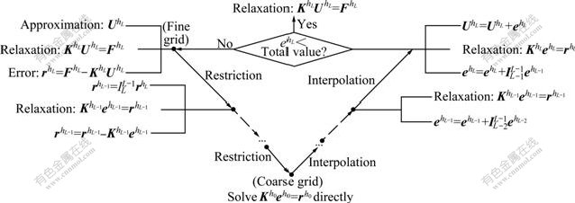
Fig.1 V-cycle based multigrid algorithm
To implement the adaptive multigrid finite element algorithm for the direct current problem, a new adaptive mesh generation strategy was defined. On a given initial mesh, the gradient recovery based a-posteriori error estimator proposed by ZIENKIEWICS and ZHU [15-16] was employed to evaluate the numerical errors. In terms of L2 norm the kth element error could be calculated,
![]()
![]() (7)
(7)
where ![]() is the gradient of element solution uh, ��e denotes the element-wise computational domain, ne means the total number of elements in the current mesh discretization, and
is the gradient of element solution uh, ��e denotes the element-wise computational domain, ne means the total number of elements in the current mesh discretization, and ![]() is the recovered gradient [17]. Based on this, the global relative error could be expressed as
is the recovered gradient [17]. Based on this, the global relative error could be expressed as
 (8)
(8)
where the global error could be obtained in the form:
![]()
Usually, the initial mesh cannot derive satisfactory results for which a new mesh is required. In the adaptive finite element process, the predicated new element size should achieve the requirement that the error distributed on each new element is equal with a specified global relative error �� being satisfied,
![]() (9)
(9)
It is known that the finite element method has a confirm convergence theorem:
![]() (10)
(10)
where p is the order of the employed shape function, which is specified as a value of 1 in our algorithm, and �� is the intensity of singularities, which is usually a value among 0.5 to 1. Then, the old element size could be resized by substituting Eqs.(7) and (9) into Eq.(10):
![]() (11)
(11)
where ![]() is the previous size of the kth element, ||e||k is the kth element error,
is the previous size of the kth element, ||e||k is the kth element error, ![]() is the gradient norm in domain ��, and ||e||�� denotes the error in domain ��.
is the gradient norm in domain ��, and ||e||�� denotes the error in domain ��.
To accelerate the convergence of the multigrid method on each adaptive refined mesh, the initial guess term was interpolated from last mesh. The whole adaptive process is displayed in Fig.2.
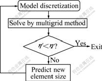
Fig.2 Flow-chart of adaptive multigrid finite element method
3 Numerical examples
To validate this proposed adaptive multigrid finite element method, the testing program based on object- oriented C++ language [19] was developed. 3-D unstructured mesh was generated by the Delaunay triangulation technique. A multigrid solver was cooperated with the well-known open source algebra multigrid iterative solver package Hypre-BloomAMG [20]. Post-processing procedures such as mesh viewing were implemented by the open source mesh package Paraview [21]. The working environment was Unix-like operating system FreeBSD with g++ compiler. All the following tests were run on a PC with Pentium-D 2.8 CPU with 512 RAM. For all the tested models the global relative error ��=10% was adopted to terminate adaptive iterative process. In addition, maximum iteration and memory cost were also used to terminate our algorithm which was specified as 5 times and 400 MB respectively.
3.1 Model 1
First, a homogeneous half-space model was considered. The background resistivity was 100 ��?m. The measuring line was 10 m in length with the interval of each potential point being 0.25 m. The current source point was located at the left-hand-side end of the measuring line with 1 A current enforced. In this model the pole-pole configuration with 41 potential points M was employed. In Fig.3, the comparison between numerical and analytical solutions is shown. On the initial mesh a standard finite element process was tested and three adaptively refined meshes (Mesh #1, #2, #3) were generated by adaptive multigrid finite element algorithm. From the results obtained from standard mesh, it can be seen that when the node distribution is not so unreasonable, larger errors basically only appear near the singularities such as the source points. As the measuring points move far away from these singularities the errors became relatively small and stable. This consequence can be explained as that the potential changes so sharply near the source points that the standard artificial mesh cannot achieve the required accuracy without mesh refinement. Moreover, the numerical results also show that the standard finite element method derive a large average relative error with a value of 3.6% and 1.8%-8.6% relative errors appear near the strong singularity areas
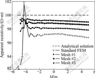
Fig.3 Apparent resistivities obtained from standard finite element method (FEM) and adaptive multigrid FEM in Model 1 (Standard FEM worked on initial mesh with 3 420 nodes and 17 910 elements; 10 364 nodes and 57 452 elements were generated in Mesh #1; 27 076 nodes and 155 751 elements were created in Mesh #2; and 64 231 nodes and 378 990 elements were generated in final Mesh #3) .
When combined with a-posteriori estimator which was employed to control iterative process, local refinement was automatically implemented. From Fig.3 it is obvious to see that singularities are gradually removed along with the mesh iterations by which the numerical results asymptotically approach the analytical ones. In the final mesh (#3) the average error is declined to 0.80% and singularity-area errors are also reduced to 0.54%-0.90%, which could be easily understood through its model discretization result in Fig.4. As for computational cost shown in Fig.5, it can be seen that the AMG solver is much superior to the well-known ICCG solver [22]. As the number of the unknowns increases during the adaptive procedure, both the iteration number and computational time consumed by ICCG solver increase dramatically; in contrast, the iteration number of AMG solver is nearly unchanged which is a value of 9-11. Based on this, the additional computational time on each iterative mesh of our adaptive multigrid algorithm is just a fraction of what the standard finite element method has cost on the initial mesh.
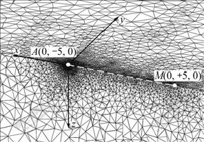
Fig.4 Final mesh generation-Mesh #3 in Model 1 by adaptive multigrid FEM
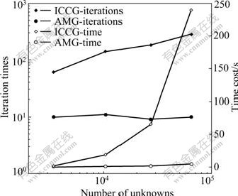
Fig.5 Efficiency comparison between ICCG and adaptive multigrid solver in Model 1
3.2 Model 2
In addition, a hemispheric model was also tested. The radius of hemisphere was 2.25 m with a resistivity of 1.0 ��?m. The background resistivity was set as 10.0 ��?m. The interval of measuring points was specified as 0.25 m with the pole-pole configuration being adopted. The current source point A was located as shown in Fig.6. From this figure, it is seen that relative errors of numerical solutions fast decrease along with the mesh adaptive refinement process (Meshes #0, #1, #2). Especially, on Mesh #2, the average relative error is reduced to 0.59% and the error near singular current source point is also confined to 0.62%-0.91%. This consequence can be explained reasonably by the final refined mesh shown in Fig.7. It is obvious to see that the intensive refinement is executed especially near the current source point, at the interfaces of anomalies and on the measuring line which is a key factor to improve the accuracy. The efficiency of AMG algorithm is displayed in Fig.8. It is clear to find that the required iteration number to solve equation exhibits an unchangeable value of 14-15 during the whole adaptive process. The additional computational time on Meshes #1 and #2 is respectively 7.4 s, which is reasonable when the increased nodes are considered.
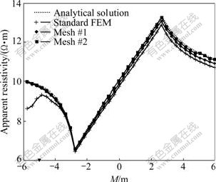
Fig.6 Apparent resistivities obtained from adaptive multigrid FEM in Model 2 (4 540 nodes and 24 431 elements were generated in initial mesh (Mesh #0); 20 060 nodes and 116 182 elements were generated in Mesh #1; 63 492 nodes and 379 122 elements were created in Mesh #2)
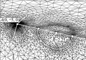
Fig.7 Final mesh generation-Mesh #2 in Model 2
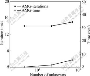
Fig.8 Performance of adaptive multigrid solver in Model 2
4 Conclusions
(1) Through combining with a-posteriori estimator, the node distribution becomes more reasonable, from which the singularities are dramatically eliminated. Moreover, some unnecessary nodes that do little contribution to improving the accuracy are avoided, which may not be implemented by the artificial work. The results obtained from Models 1 and 2 also show that adaptive multigrid finite element method can converge to the exact solution quickly with no more than four iterations, which is also essential for the inversion since it may need a lot of forward modeling iterations to obtain the final results. In the whole process, no interference is needed, which cannot be obtained by standard finite element procedures.
(2) Compared with the well-known ICCG solver, the efficiency of our adaptive multigrid solver is validated. As the nodes increase and accuracy are considered, the additional cost spent on solving each iterative linear equation is reasonably small, by which the efficiency and robustness of our adaptive multigrid finite element algorithm is remarkably demonstrated.
(3) Although the algorithm is only tested on DC resistivity examples, its application potential to other geophysical field can be predicted.
Acknowledgments
Dr. REN thanks China Scholarship Council 2008 project for a four- year PhD grant in ETH-Zurich and Dr. GUO thanks CSC 2007 project for a two-year joint-PhD grant between Central South University and University of Victoria. The authors give special thanks to Dr. R?ECKER (University of Leipzig, Germany) and Professor HVOZDARA (Geophysical Institute, Slovak Academy of Sciences) to provide fruitful discussion. And the authors also give honored thanks to Hypre and Paraview teams for freely opening their state of the art packages.
References
[1] LI Y G, SPITZER K Three-dimensional DC resistivity forward modelling using ?nite elements in comparison with ?nite-difference solutions [J]. Geophys J Int, 2002, 151: 924-934.
[2] ZHOU B, GREENHALGH S A. Finite element three-dimensional direct current resistivity modelling: Accuracy and ef?ciency considerations [J]. Geophys J Int, 2001, 145: 679-688.
[3] WU Xiao-ping. A 3-D finite-element algorithm for DC resistivity modelling using the shifted incomplete Cholesky conjugate gradient method [J]. Geophys J Int, 2003, 154: 947-956.
[4] SHEN Jin-song, SUN Wen-bo. 2.5-D modeling of cross-hole electromagnetic measurement by finite element method [J]. Pet Sci, 2008, 5: 126-134.
[5] XIONG Bin, LUO Yan-zhong. Finite element modeling of 2.5-D TEM with blocks homogeneous conductivity [J]. Chinese Journal Geophysics, 2006, 49(2): 590-597. (in Chinese)
[6] FENG T, GULLIKSSON M, LIU W B. Adaptive finite element methods for the identi?cation of elastic constants [J]. Journal of Scienti?c Computing, 2006, 26(2): 217-235.
[7] MOLLER M, KUZMIN D. Adaptive mesh refinement for high-resolution finite element schemes [J]. Int J Numer Meth Fluids, 2006, 52: 545-569.
[8] KERRY K, CHESTER W. Adaptive finite-element modeling using unstructured grids: The 2D magnetotelluric example [J]. Geophysics, 2006, 71(6): G291-G299.
[9] LI Y G, KERRY K. 2D marine controlled-source electromagnetic modeling: Part 1. An adaptive finite-element algorithm [J]. Geophysics, 2007, 72(2): WA51-WA62.
[10] STEPHAN P, MAISCHAK M, LEYDECKER F. An hp-adaptive ?nite element/boundary element coupling method for electromagnetic problems [J]. Comput Mech, 2007, 39: 673-680.
[11] TANG Jing-tian, REN Zheng-yong, HUA Xi-rui. Theoretical analysis of geo-electromagnetic modeling on Coulomb gauged potentials by adaptive finite element method [J]. Chinese Journal Geophysics, 2007, 50(5): 1584-1597. (in Chinese)
[12] WILLIAM L B. A multigrid tutorial [M]. 2nd ed. Philadelphia: Society for Industrial and Applied Mathematics, 2000.
[13] CHEN Z M, WANG L, ZHENG W Y. An adaptive multigrid method for time-harmonic Maxwell equations with singularities [J]. SIAM Journal Science Computation, 2007, 20(1): 118-139.
[14] MULDER W A. A multigrid solver for 3D electromagnetic diffusion [J]. Geophysical Prospecting, 2006, 54: 633-649.
[15] ZIENKIEWICZ O C, ZHU J Z. Super-convergent patch recovery and a posteriori error estimates: Part 1. The recovery technique [J]. International Journal in Numerical Method Engineering, 1992, 33(7): 1331-1364.
[16] ZIENKIEWICZ O C, ZHU J Z. Super-convergent patch recovery and a posteriori error estimates: Part 2. Error estimates and adaptivity [J]. International Journal in Numerical Method Engineering, 1992, 33(7): 1365-1382.
[17] ZIENKIEWICZ O C, TAYLOR R L. The finite-element method [M]. Butterworth-Heinemann: Elsevier, 2000.
[18] JIN J. The finite element method in electromagnetics [M]. New York: John Wiley & Sons, 2001.
[19] REN Zheng-yong, TANG Jing-tian. Object-oriented philosophy in designing adaptive finite-element package for 3D elliptic deferential equations [J]. EOS on Transactions, 2007, 88(52): NS11A-0164.
[20] HYPRETEAM. Hypre: A high performance preconditioner [EB/OL]. [2007-01-04]. http://www.llnl.gov/CASC/hypre/.
[21] PARAVIEWTEAM. Paraview: An open-source multi-platform parallel visualization application [EB/OL]. [2008-06-09]. http:// www.paraview.org/New/index.html.
[22] RICHARD B, MICHAEL B, TONY F C, DEMMEL J, DONATO J M, DONGARRA J, EIJKHOUT V, POZO R, ROMINE C, van der VORST H. Templates for the solution of linear systems, building blocks for iterative methods [M]. New York: Society for Industrial and Applied Mathematics, 2006.
Foundation item: Projects(2006AA06Z105, 2007AA06Z134) supported by the National High-Tech Research and Development Program of China; Projects(2007, 2008) supported by China Scholarship Council (CSC)
Received date: 2009-05-23; Accepted date: 2009-09-04
Corresponding author: REN Zheng-yong, Doctoral candidate; Tel: +86-731-88877973; E-mail: renzhengyong@gmail.com
Abstract: Based on the fact that 3-D model discretization by artificial could not always be successfully implemented especially for large-scaled problems when high accuracy and efficiency were required, a new adaptive multigrid finite element method was proposed. In this algorithm, a-posteriori error estimator was employed to generate adaptively refined mesh on a given initial mesh. On these iterative meshes, V-cycle based multigrid method was adopted to fast solve each linear equation with each initial iterative term interpolated from last mesh. With this error estimator, the unknowns were nearly optimally distributed on the final mesh which guaranteed the accuracy. The numerical results show that the multigrid solver is faster and more stable compared with ICCG solver. Meanwhile, the numerical results obtained from the final model discretization approximate the analytical solutions with maximal relative errors less than 1%, which remarkably validates this algorithm.
