J. Cent. South Univ. (2017) 24: 227-235

DOI: 10.1007/s11771-017-3423-y

Robust elastic impedance inversion using L1-norm misfit function and constraint regularization

PAN Xin-peng(潘新朋)¹, ZHANG Guang-zhi(张广智)^{1, 2}, SONG Jia-jie(宋佳杰)¹, ZHANG Jia-jia(张佳佳)^{1, 2},

WANG Bao-li(王保丽)^{1, 2}, YIN Xing-yao(印兴耀)^{1, 2}

1. School of Geosciences, China University of Petroleum (Huadong), Qingdao 266580, China;

2. Laboratory for Marine Mineral Resources, Qingdao National Laboratory Marine Science and Technology,

Qingdao 266071, China

 Central South University Press and Springer-Verlag Berlin Heidelberg 2017

Abstract:

The classical elastic impedance (EI) inversion method, however, is based on the L2-norm misfit function and considerably sensitive to outliers, assuming the noise of the seismic data to be the Guassian-distribution. So we have developed a more robust elastic impedance inversion based on the L1-norm misfit function, and the noise is assumed to be non-Gaussian. Meanwhile, some regularization methods including the sparse constraint regularization and elastic impedance point constraint regularization are incorporated to improve the ill-posed characteristics of the seismic inversion problem. Firstly, we create the L1-norm misfit objective function of pre-stack inversion problem based on the Bayesian scheme within the sparse constraint regularization and elastic impedance point constraint regularization. And then, we obtain more robust elastic impedances of different angles which are less sensitive to outliers in seismic data by using the IRLS strategy. Finally, we extract the P-wave and S-wave velocity and density by using the more stable parameter extraction method. Tests on synthetic data show that the P-wave and S-wave velocity and density parameters are still estimated reasonable with moderate noise. A test on the real data set shows that compared to the results of the classical elastic impedance inversion method, the estimated results using the proposed method can get better lateral continuity and more distinct show of the gas, verifying the feasibility and stability of the method.

Key words:

elastic impedance (EI) inversion; L1-norm misfit function; sparse constraint regularization; elastic impedance point constraint regularization; IRLS strategy；

1 Introduction

Geophysical inversion problems are considered as optimization problems in general, in which the goal is to find a solution that minimizes the misfits. The classical least-squares (LS) criterion is based on the L2-norm misfit minimization, but it tends to overestimate the influence of outliers in real seismic data. So, the noise in seismic data is beyond description with the Gaussian distribution when outliers abound in seismic data, and the robustness of inversion must be taken into consideration now. Instead, the least-absolute-values criterion based on the L1-norm misfit minimization is known to be insensitive to outliers, which it corresponds to the solution of minimum median error affected little by outliers, and may yield more stable estimated value than the L2-norm misfit minimization does [1-5]. However, the inversion problem based on the L1-norm optimization is obviously nonlinear and may bring higher computational cost [6]. Many scholars have studied the method to solve the problem, including the linear programming method, the interior-point method and the iteratively re-weighted least square (IRLS) method [7-9].

Moreover, the seismic inversion problem is an ill-posed problem because of the noisy seismic data, the band-limited wavelet or other reasons. And the most effective way to solve ill-posed problems is the regularization methods assisted with proper optimization techniques [10-12]. To stabilize the inversion via the inclusion of a priori constraint, we attend to apply the statistical Bayesian approach to combine the observed data with the available prior information to get a more stable inversion solution [13], and therefore we attempt to treat the long-tailed Cauchy probability distribution as a priori information [14-16]. Compared to the Gaussian probability distribution, the Cauchy probability distribution as a prior has long tails, resulting in a regularization term that produces sparse solutions. On account of the band-limited characteristics of the real seismic data, a prior information constraint coming from the logging data, the geological horizons or other information can be used for a regularization term to guarantee that the inverted values include low-frequency information [17]. But what I want to emphasize is this: for the one-dimensional data, we can take advantage of the known points to constraint the final inversion results; for the two-dimensional data or the three-dimensional data, we should choose an interpolation scheme to interpolate the known points, and the most common way is to use the logging data interpolating along the geological horizons to improve the lateral continuity of the inversion results. In this work, we will append the sparse constraint regularization and elastic impedance point constraint regularization to make the inversion results more robust and stable.

Elastic impedance (EI) concept was first introduced by CONNOLLY [18], and WHITCOMBE [19] had proposed a normalized EI equation to deal with the dimensionality problem. Nowadays, the EI inversion has been widely used in industry. The classical EI inversion method, however, is based on the L2-norm misfit minimization and considerably sensitive to outliers, so we have developed a more robust elastic impedance inversion method based on the L1-norm misfit minimization and two regularization methods including the sparse constraint regularization term and elastic impedance point constraint regularization term. Firstly, we create the objective function of seismic inversion based on the Bayesian scheme to combine the observed data with a priori information. And then, we invert the elastic impedance of different angles based on L1-norm misfit minimization and regularization methods by using the IRLS strategy. Finally, we extract the P-wave and S-wave velocity and density via the elastic impedance equation proposed by CONNOLLY [18] and WHITCOMBE [19]. Through the designed one-dimensional impedance layered model, we make an attempt to compare the impedance inversion method based on the L1-norm misfit function and constraint regularization with the classical impedance inversion method to validate the robustness and the anti-noise characteristics of the method proposed in our paper. Tests on synthetic data show that the P-wave and S-wave velocity and density parameters are still estimated reasonable with moderate noise. Meanwhile, a test on the real data set shows that compared to the results of the classical elastic impedance inversion method, the estimated results using the method proposed in this paper are in good agreement with the results of drilling, and can also get better lateral continuity and more distinct show of the gas, verifying the feasibility and stability of the method proposed in this paper.

2 Theory

2.1 Objective function

Bayesian theory can provide a theoretical framework to make probabilistic estimates combining observed data and a priori information. And the resulting probabilistic parameter estimates are called the Posterior Probability Distribution Function (PPDF). Following ULRYCH et al [20] and DOWNTON [14], the Bayesian theory estimates the PPDF via the likelihood function  and a priori probability function p(r), which can be expressed as

                        (1)

where  suggests the probability of the reflection coefficient vector r given the seismic data vector d. The denominator P(d) is a normalization function when may be ignored when only the shape of the PPDF is considered, so

                        (2)

Assuming that seismic convolution model is

                         (3)

where r denotes the seismic sparse reflection sequence; d denotes the noisy seismic data, and the noise n is assumed to be non-Gaussian; G is the wavelet matrix. Following GERSZTENKORN et al [21], the likelihood function for L1-norm can be expressed as

          (4)

where f_m(r) describes the functional relationship between the observed seismic data d_m and reflection sequence r; σ denotes the standard deviation of seismic noise. To stabilize the inversion via the inclusion of a priori information, we attend to apply the statistical Bayesian approach to combine the observed data with the available prior information. Assuming the reflection sequence may be modeled as a long tailed distribution, such as the L1-norm distribution [6], the Huber norm distribution [22], the biweight norm distribution [5] or Cauchy distribution [14]. Here, we use the Cauchy distribution as the sparse constraint regularization, which is expressed as

                         (5)

So, the PPDF  can be expressed via Bayesian theory as

       (6)

It is easier to take the partial derivatives of the logarithm of the function:

         (7)

As for the one-dimensional data, we can use the known points to constraint the final inversion results. And in the case of the two-dimensional data or the three- dimensional data, however, the most common way is to use the logging data interpolating along the geological horizons to improve the lateral continuity of the inversion results. To ensure that the inverted parameters could include the low frequency information, we append the elastic impedance point constraint regularization as the model constraint [17]. So, the objective function is

                  (8)

Three parts are included in equation 8: J_L1(r) represents the difference between the synthetic data and the observed data; J_Cauchy(r) represents the prior Cauchy distribution sparse constraint regularization; and J_EI(r) represents the elastic impedance point constraint regularization. Where EI(θ, t₀) represents the initial elastic impedance;  represents the integral operator matrix;λ_e represents the elastic impedance point constraint regularization factor, controlling the accuracy and stability of the inversion results.

2.2 IRLS algorithm to solve objective function

According to the derivation of objective function, the partial derivative of the objective function is

        (9)

So, it results in

 (10)

where

;

;

Θ is the sparse constraint regularization factor to control the sparseness of reflection sequence; σ_r is the standard deviation of reflection sequence; W_L1 is the misfit weighting function, where ε<<1 is a small  number to protect against the singularity that arises for

Because of the introduce of misfit weighting function W_L1 and the Cauchy sparse constraint regularization term ΘQ, Eq. (10) is a nonlinear equation and cannot be easy to be solved via the linear algorithms. One of the most efficient ways is the IRLS algorithm, and it can deal with the weighting problem and solve the nonlinear equation iteratively. Given the initial reflection sequence r₀, we can obtain the misfit weighting function W_L1 and Cauchy sparse constraint regularization ΘQ_e via their expression. Then, solve the equation 10 by using the conjugate gradient algorithm [23] to obtain the updated reflection sequence r₁ and corresponding W_L1 and ΘQ_e. This process is iteratively operated until

satisfying the convergence condition , where ξ is a tolerance value [6].

So, we can obtain the elastic impedance of different angles by using path integral method expressed as

           (11)

2.3 Robustness validation of impedance inversion based on L1-norm misfit function and constraint regularization

To validate the robustness and the anti-noise characteristics of elastic impedance inversion method based on the L1-norm misfit function and constraint regularization, we design a one-dimensional impedance layered model shown in Fig. 2 plotted with black solid line, and make an attempt to compare the method proposed in our paper with the classical impedance inversion method. The seismic data shown in Fig. 1 are generated by convolving the three angle reflection coefficients according to the expression of CONNOLLY [18] with a Ricker wavelet whose dominant frequency is 40 Hz. Then, 20% Gaussian random noise and some outliers plotted with green squares are added into the seismic data, as shown in Fig. 1. We just do the inversion of the middle angle gather for the sake of brevity, and a priori model plotted in green shown as Fig. 2 is the same for both the two inversion method. The final results of two inversion method plotted with blue and red dashed lines are shown as Fig. 2.

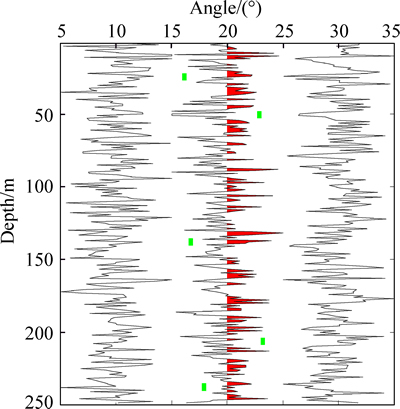
Fig. 1 Seismic angle gathers including 10°, 20° and 30° with 20% Gaussian random noise and five outliers

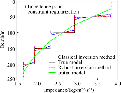
Fig. 2 Comparison of robust impedance inversion method and classical impedance inversion method in noise situation

From Fig. 2, we find that with the impedance point constraint regularization, the result of robust impedance inversion method based on the L1-norm misfit function is much better than that of the classical impedance inversion method and is closer to the true model, so the robust impedance inversion method may be more robust than the classical method when some outliers exist in the seismic data. In particular, the elastic impedance point constraint regularization in the real data example can significantly improve the lateral continuity of seismic sections, and enhance the stability of the inversion results. Meanwhile, assuming the reflection sequence is modeled as a long tailed Cauchy distribution, so the final result shows better.

2.4 Parameter extraction based on inverted elastic impedance

The elastic impedance, or EI, function was first proposed by CONNOLLY [18], and the expression is

        (12)

where  However, an undesirable feature of the EI function has been that its dimensionality varies with incidence angle θ and provides numerical values that change significantly with θ. So, WHITCOMBE et al [19] had proposed the normalized elastic impedance to solve the problem, in which the modifications neither improve nor degrade the accuracy of the reflectivity that can be derived from the EI function. And its expression is

                    (13)

So, we can extract the parameter directly based on the relationship between the elastic impedance and elastic parameters including the P- and S-wave velocity and density. To solve the nonlinear Eq. (13), we adopt the logarithm process to get the linear formula expressed as

                       (14)

where  Then, we solve the equation 14 to obtain the weighting coefficient a(θ), b(θ), c(θ) of the incidence angle θ via the least square (LS) method or singular value decomposition (SVD) method, where the elastic impedance EI(t, θ) uses the inverted EI results of seismic traces near wells, and ρ(t), V_p(t), V_s(t) use the logging data, which could be processed by Backus averaging to keep the unification between the seismic data and logging data [24].

Aiming at three different incidence angles, we can obtain nine coefficients including a(θ₁), b(θ₁), c(θ₁); a(θ₂), b(θ₂), c(θ₂); a(θ₃), b(θ₃), c(θ₃), and then we can get lnρ(t), lnV_p(t), lnV_s(t) through the equation expressed as

 (15)

So, we can obtain the P-wave and S-wave velocity and density at any sampling point.

3 Example

3.1 Synthetic test

To test the feasibility of the robust elastic impedance inversion method using L1-norm misfit function, the sparse constraint regularization and elastic impedance point constraint regularization, we carry out the feasibility and noise immunity test of A well in one work area.

As shown in Fig. 3(a) and Fig. 6(a), we apply well log data to make synthetic seismogram in noise and noise-free situations, and then invert elastic impedance of three angles based on the robust elastic impedance inversion method for the direct extraction of P-wave and S-wave velocity and density parameter, testing the feasibility and noise immunity of the method.

From Figs. 4 and 5, we find that both the inverted elastic impedance of three angles and the extracted P-wave and S-wave velocity and density in noise-free situation are consistent with the true values, and synthetic angle gathers using these inverted results produce fewer errors compared with real angle gathers shown as Fig. 3(b), so the robust elastic impedance inversion method using L1-norm misfit function, the sparse constraint regularization and elastic impedance point constraint regularization is feasible.

From Figs. 7 and 8, we find that when adding random noise in SNR=3 to the synthetic seismograms shown as Fig. 6(a), both the inverted elastic impedance of three angles and the extracted P-wave and S-wave velocity and density in noise situation are also consistent with the true values, therefore, it validates the robustness and noise immunity of the method of robust elastic impedance inversion using L1-norm misfit function, the sparse constraint regularization and elastic impedance point constraint regularization, and the inverted parameters are relatively accurate, which can reflect the major characteristics of oil-bearing reservoir well.

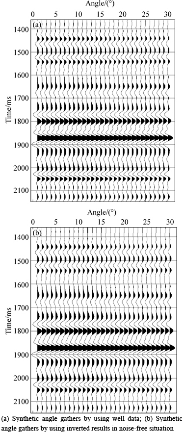
Fig. 3 Comparison of synthetic angle gathers using well log data and gathers by using inverted results in noise-free situation:

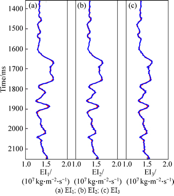
Fig. 4 Inverted elastic impedance results of three angles by using the robust elastic impedance inversion method in noise-free situation (blue and red solid lines indicate true values and inverted results respectively):

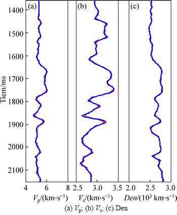
Fig. 5 Extracted P-wave and S-wave velocity and density in noise-free situation (blue and red solid lines indicate true values and extracted results respectively):

3.2 Real data

Real data are used to validate the applicability of the robust elastic impedance inversion method using L1-norm misfit function, the sparse constraint regularization and elastic impedance point constraint regularization. Case studies from the colony sand in Alberta, a Gulf coast sand, offshore eastern Canada Whiterose field [25], and three partial angle-stack seismic profiles ranging from 0.6 s to 0.7 s are shown in Fig. 9. As shown in Fig. 9, the logging interpretation results indicate that the gas reservoir discoveries in green solid ellipse. Within the Colony formation, thin sands are developed and can produce commercial gas where they are structurally high, and the well shown in the following figures was drilled on the gas-filled anomalies in the Colony formation [26]. Then, we build a priori model by using the logging data under the constraints of geologic horizons, and perform our inversion method proposed in this paper on the real data. In the end, the inverted elastic impedance of three angles and the extracted P-wave and S-wave velocity and density are displayed in Figs. 10 and 11, respectively. We also perform a classical elastic impedance inversion method proposed by CONNOLLY [18] and WHITCOMBE et al [19] on the real data, and the extracted P-wave and S-wave velocity and density are displayed in Fig. 12.

Fig. 6 Comparison of synthetic angle gathers using well log data and gathers by using inverted results in noise situation (SNR=2):

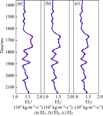
Fig. 7 Inverted elastic impedance results of three angles by using robust elastic impedance inversion method in noise situation (SNR=2) (blue and red solid lines indicate true values and inverted results respectively):

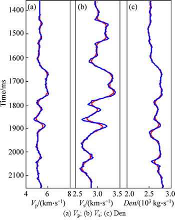
Fig. 8 Extracted P-wave and S-wave velocity and density in noise situation (SNR=2) (blue and red solid lines indicate true values and extracted results respectively):

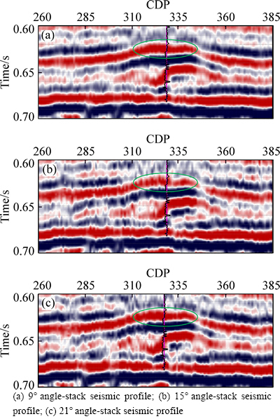
Fig. 9 Angle-stack seismic profiles with three different angles:

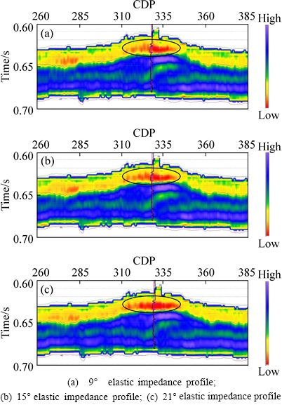
Fig. 10 Inverted elastic impedance profiles using robust elastic impedance inversion method proposed:

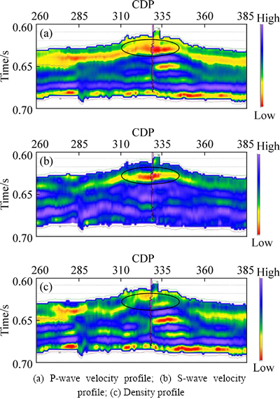
Fig. 11 Extracted P-wave and S-wave velocity and density profiles using robust elastic impedance inversion method proposed:

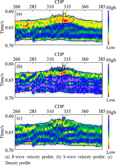
Fig. 12 Extracted P-wave and S-wave velocity and density profiles using classical elastic impedance inversion method:

From Fig. 10, we find that the inverted elastic impedance profiles based on the robust elastic impedance inversion method with three different angles is highly precise, which show low value and agree with the results of oil-bearing reservoir in logging interpretation.

Gas within the Colony sand is seismically detectable owing to the relatively low velocity of the gas sand [26]. Figure 11 shows that the extracted P-wave and S-wave velocity is also consistent with the results in logging interpretation, which presenting low values and reflecting the characteristics of gas-bearing reservoir obviously. Compared to the results using the classical elastic impedance inversion method, the extracted P-wave and S-wave velocity profiles using the robust elastic impedance inversion method proposed in this paper get better lateral continuity and more distinct show of the gas, verifying the feasibility and stability of the method proposed in this paper. However, the extracted density is not perfect compared to the other extracted P-wave and S-wave velocity, as the incidence angle of seismic data is relatively small and the density term inversion has to need the information of long offset. Anyway, it further validates the availability of the robust elastic impedance inversion method using L1-norm misfit function, the sparse constraint regularization and elastic impedance point constraint regularization, which is promising in practical applications.

4 Conclusions

We introduce a more robust elastic impedance inversion method using L1-norm misfit function, the sparse constraint regularization and elastic impedance point constraint regularization. Based on the Bayesian framework, we first derive the objective function based on L1-norm misfit function with the sparse constraint regularization and elastic impedance point constraint regularization. Then we apply the IRLS algorithm to solve the nonlinear objective function to obtain more robust elastic impedances of different angles which are less sensitive to outliers in seismic data. Finally, we get the P-wave and S-wave velocity and density with the more stable parameter extraction method. Through the designed one-dimensional impedance layered model, we find the robustness and the anti-noise characteristics of the method proposed in our paper is better than the classical impedance inversion method. Compared to the results of the classical elastic impedance inversion method, the estimated results using the method proposed in this paper are in good agreement with the results of drilling, and can also get better lateral continuity and more distinct show of the gas, verifying the robust elastic impedance using L1-norm misfit function, the sparse constraint regularization and elastic impedance point constraint regularization. Of course, the inverted density result of real data shows that we have to use relatively large incidence angle data to obtain a more accurate density parameter.

It is well known that reservoir fluid identification is very important, and the extraction of effective fluid identification factor is necessary. Hence, the next study which we want to attempt is to find a useful fluid identification factor and extract it directly by using the robust elastic impedance inversion method. And we will also use the large incidence angle data to obtain more accurate density parameter.

References

[1] CLAEROUT J F, MUIR F. Robust modeling with erratic data [J]. Geophysics, 1973, 38(5): 826-844.

[2] TAYLOR H L, BANKS S C, MCCOY J F. Deconvolution with the L-one norm [J]. Geophysics, 1979, 44(1): 39-52.

[3] TARANTOLA A. Inverse problem theory, methods for data fitting and model parameter estimation [M]. New York: Elsevier Science Publishers, 1987.

[4] SCALES J A, GERSZTENKOR N. Robust methods in inverse theory [J]. Inverse Problems, 1988, 4: 1071-1091.

[5] JI J. Robust inversion using biweight norm and its application to seismic inversion [J]. Exploration Geophysics, 2012, 43(2): 70-76.

[6] ZHANG F C, DAI R H, LIU H Q. Seismic inversion based on L1-norm misfit function and total variation regularization [J]. Journal of Applied Geophysics, 2014, 109: 111-118.

[7] SAFON C, VASSEUR G, CUER M. Some applications of linear programming to the inverse gravity problem [J]. Geophysics, 1977, 42(6): 1215-1229.

[8] DAUBECHIES I, DEVORE R, FORNASIER M, GUNTURK C S. Iteratively reweighted least squares minimization for sparse recovery [J]. Communications on Pure and Applied Mathematics, 2010, 63: 1-38.

[9] ASTER R C, BORCHERS B, THURBER C H. Parameter estimation and inverse problems [M]. 2nd edition. New York: Elsevier Academic Press, 2013.

[10] TIKHONOV A N, ARSENIN V Y. Solutions of ill-posed problems [J]. Mathematics of Computation, 1977, 32(144): 1320-1322.

[11] TIKHONOV A N, GONCHARSKY A V, STEPANOV V V, YAGOLA A G. Numerical methods for the solution of ill-posed problems [M]. New York: Mathematics and Its Applications, 1995.

[12] WANG Y F. Seismic impedance inversion using l₁-norm regularization and gradient descent methods [J]. J Inv Ill-Posed Problems, 2011, 18: 823-838.

[13] BULAND A, OMRE H. Bayesian linearized AVO inversion [J]. Geophysics, 2003, 68(1): 185-198.

[14] DOWNTON J E. Seismic parameter estimation from AVO inversion [D]. Calgary: University of Calgary, 2005.

[15] THEUNE U, JENSAS I, EIDSIVIK J. Analysis of prior models for a blocky inversion of seismic AVA data [J]. Geophysics, 2010, 75(3): 25-35.

[16] ALEMIE W, SACCHI M D. High-resolution three-term AVO inversion by means of a trivariate Cauchy probability distribution [J]. Geophysics, 2011, 76(3): 43-55.

[17] ZONG Z Y, YIN X Y, WU G C. Elastic impedance parameterization and inversion with Young’s modulus and Poisson’s ratio [J]. Geophysics, 2013, 78(6): 35-42.

[18] CONNOLLY P. Elastic impedance [J]. The Leading Edge, 1999, 18(4): 438-452.

[19] WHITCOMBE D N. Elastic impedance normalization [J]. Geophysics, 2002, 67(1): 60-62.

[20] ULRYCH T J, SACCHI M D, WOODBURY A. A Bayes tour of inversion: A tutorial [J]. Geophysics, 2001, 66(1): 55-69.

[21] GERSZTENKORN A, BEDNAR J B, LINES L R. Robust iterative inversion for the one-dimensional acoustic wave equation [J]. Geophysics, 1986, 51(2): 357-368.

[22] GUITTON A, SYNES W W. Robust inversion of seismic data using the Huber norm [J]. Geophysics, 2003, 68(4): 1310-1319.

[23] TARANTOLA A. Inverse problem theory and methods for model parameter estimation [M]. New York: Society for Industrial Mathematic, 2005.

[24] LINDSAY R, KOUGHNET V. Sequential Backus averaging: upscaling well logs to seismic wavelengths [J]. The Leading Edge, 2001, 20(2): 188-191.

[25] ROYLE A J. Exploitation of an oil field using AVO and post-stack rock property analysis methods [J]. CREWES Research Report, 2001, 13-17.

[26] FOCHT G W, BAKER F E. Geophysical case history of the two hills colony gas field of alberta [J]. Geophysics, 1985, 50(7): 1061-1076.

(Edited by DENG Lü-xiang)

Cite this article as: PAN Xin-peng, ZHANG Guang-zhi, SONG Jia-jie, ZHANG Jia-jia, WANG Bao-li, YIN Xing-yao. Robust elastic impedance inversion using L1-norm misfit function and constraint regularization [J]. Journal of Central South University, 2017, 24(1): 227-235. DOI: 10.1007/s11771-017-3423-y.

Foundation item: Projects(U1562215, 41674130, 41404088) supported by the National Natural Science Foundation of China; Projects(2013CB228604, 2014CB239201) supported by the National Basic Research Program of China; Projects(2016ZX05027004-001, 2016ZX05002006-009) supported by the National Oil and Gas Major Projects of China; Project(15CX08002A) supported by the Fundamental Research Funds for the Central Universities, China

Received date: 2015-08-08; Accepted date: 2016-01-05

Corresponding author: ZHANG Guang-zhi, Professor, PhD; Tel: +86-15953229862; E-mail: zhanggz@upc.edu.cn

Abstract: The classical elastic impedance (EI) inversion method, however, is based on the L2-norm misfit function and considerably sensitive to outliers, assuming the noise of the seismic data to be the Guassian-distribution. So we have developed a more robust elastic impedance inversion based on the L1-norm misfit function, and the noise is assumed to be non-Gaussian. Meanwhile, some regularization methods including the sparse constraint regularization and elastic impedance point constraint regularization are incorporated to improve the ill-posed characteristics of the seismic inversion problem. Firstly, we create the L1-norm misfit objective function of pre-stack inversion problem based on the Bayesian scheme within the sparse constraint regularization and elastic impedance point constraint regularization. And then, we obtain more robust elastic impedances of different angles which are less sensitive to outliers in seismic data by using the IRLS strategy. Finally, we extract the P-wave and S-wave velocity and density by using the more stable parameter extraction method. Tests on synthetic data show that the P-wave and S-wave velocity and density parameters are still estimated reasonable with moderate noise. A test on the real data set shows that compared to the results of the classical elastic impedance inversion method, the estimated results using the proposed method can get better lateral continuity and more distinct show of the gas, verifying the feasibility and stability of the method.