

J. Cent. South Univ. (2018) 25: 2641-2653
DOI: https://doi.org/10.1007/s11771-018-3942-1

Dynamic model for internally carried air-launched rocket
ZHENG Wu-ji(֣��), ZHANG Deng-cheng(�ŵdz�)
Aeronautics Engineering College, Air Force Engineering University, Xi��an 710038, China
 Central South University Press and Springer-Verlag GmbH Germany, part of Springer Nature 2018
Abstract:
For rigid-flexible coupling multi-body with variable topology, such as the system of internally carried air-launched or heavy cargo airdrop, in order to construct a dynamic model with unified form, avoid redundancy in the modeling process and make the solution independent, a method based on the equivalent rigidization model was proposed. It divides a system into independent subsystems by cutting off the joints, of which types are changed with the operation process of the system. And models of different subsystems can be constructed via selecting suitable modeling methods. Subsystem models with flexible bodies are on the basis of the equivalent rigidization model which replaces the flexible bodies with the virtual rigid bodies. And the solution for sanction, which is based on the constraints force algorithm (CFA) and vector mechanics, can be independent on the state equations. The internally carried air-launched system was taken as an example for verifying validity and feasibility of the method and theory. The dynamic model of aircraft-rocket-parachute system in the entire phase was constructed. Comparing the modeling method with the others, the modeling process was programmed; and form of the model is unified and simple. The model, method and theory can be used to analyze other similar systems such as heavy cargo airdrop system and capsule parachute recovery system.
Key words:
Cite this article as:
ZHENG Wu-ji, ZHANG Deng-cheng. Dynamic model for internally carried air-launched rocket [J]. Journal of Central South University, 2018, 25(11): 2641�C2653.
DOI:https://dx.doi.org/https://doi.org/10.1007/s11771-018-3942-11 Introduction
So far, the research on internally carried air-launched rocket and heavy-equipment airdrop at home and abroad mainly concentrates on the modeling and simulation [1�C5], the design of control laws [6], the airdrop experiments [7, 8], the analysis of stability and maneuverability, and the development of air launch and precision airdrop technology [9�C14]. But up to now, there hasn��t been accepted model of the systems above. As we all know, the internally carried air-launched system is a complex parachute-payload system with variable topology, which is similar to a typical HCADS (Heavy Cargo Airdrop System) [3] and CPAS (Capsule Parachute Recovery System) [15�C17]. Multi-body system, such as air-launched system, consists of interconnected components, and flexible parts often exist in such a system [18], and the fluid structure interaction of the parachutes and other parts of the system is most complex [19], and they make modeling and analysis very difficult. In order to reduce the problem to one of an appropriate size, some researchers made the rigid assumptions, which could cause more errors in actual conditions. As time goes by, several approaches have been proposed to treat large elastic deformations of flexible multi-body systems. Some researchers [15] split the deploying suspensions and parachute into N rigid links, thus the deploying parachute system can be regarded as an open chain multi-body system,in which each body is connected by means of revolute joints. Others [15, 20] used mass spring damper model, in which suspensions line and main canopy were modeled as serials lumped mass connected to each other by springs. More details about the models can be seen in Ref. [15].
However, because flexible bodies exist in the system and the methods for rigid body are different from those of flexible body, the dynamic equations for rigid-flexible coupling multi-body system cannot be constructed at the same time and solved independently, which makes modeling process more complex and redundant. Moreover, considering that the topology of the multi-body systems is changed with the operation process of system and the generalized coordinates are different for different topologies, the models cannot be easily established via only one modeling method such as Kane method [21, 22] or analytical mechanism [23, 24], which is based on the selection of suitable generalized coordinates to simplify modeling process. Furthermore, the forms of the models in different phases are always not unified. For examples, some researchers assumed that the position and rotation of the aircraft in airdrop phase were pre-determined and did not result from forces and moments acting upon it. Others [5, 23] assumed that the parachute model was simplified as drag, which run opposite of the airflow axis. And the total airdrop lifetime was divided into some phases and the models in different phases were constructed separately [3].
To surmount these flaws, this paper proposed the equivalent rigidization model, which made modeling process of rigid body and flexible body unified. And based on the equivalent rigidization model, constraints force algorithm (CFA) [15], vector mechanism [25] and rigid modeling method, this paper proposed a method to construct a unified model for the rigid-flexible coupling multi-body with variable topology, which achieved the goal of unified modeling process and independent solution. To verify the veracity and feasibility of the above method and theory, we took internally carried air-launched rocket as an example, and then a virtual simulation system for the characteristic research of air-launched system was developed through MATLAB/Simulink, C language and ADAMS (a dynamic software). This model, method and theory can serve as the foundation for the subsequent quantitative research.
2 Equivalent rigidization of flexible body
2.1 Movement description of flexible suspension line
The suspension line and its frame are described in Figure 1. As shown in Figure 1, s is the Lagrange arc length coordinate before suspension line��s deformation and s1 is the Lagrange arc length coordinate after the suspension line��s deformation. Base on the French frame (t, n, b), the origin of the local frame Otxtytzt is at the center of the differential element, while the zt-axis points forward and parallels to the tangent vector t, the yt-axis points upward in the vertical plane and parallels to the principal normal n and the xt-axis points left and parallels to the subnormal b. In order to reduce the problem to one of an appropriate size, a number of simplifying assumptions have been made.
1) Suspension line is a flexible body, which is homogeneous, continuous and isotropic.
2) The shear force and horizontal moment of suspension line are negligible.
3) Axial displacement of suspension line is small enough, and defined as 
 .
.
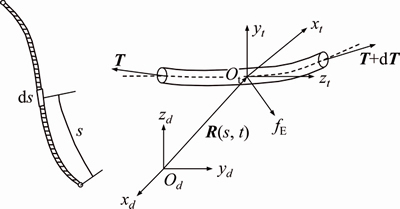
Figure 1 Differential element and its local frame
As a flexible body, suspension line cannot endure shear force and moment, so the internal force only refers to stretching force. The transformation matrix B(s,t) from a vector in the local frame to the inertial reference frame can be described by a rotation by Euler angles of �� and f.
 (1)
(1)
The tangent vector t at s position can be expressed as
 (2)
(2)
The stiffness of suspension line is employed EA. Using it and based on the linear elastic hypothesis, we can get the stretching force:
 (3)
(3)
The velocity of suspension line in the local frame can be given by
 (4)
(4)
Based on the theory of conservation of mass, the relation between ��l and ��l* can be given by
 (5)
(5)
where ��l is density below displacement; ��l* is density after displacement.
Defining ��(s,t) as the angular velocity of differential element in the local frame and ��(s,t) as the suspension line curvature in the local frame and using Figure 1, we find the following relations:
 (6)
(6)
 (7)
(7)
2.2 Continuous model
Based on the Newton��s Second Law of motion, all the differential elements (ds) meet the following vector equation,
 (8)
(8)
where f is distributed loading which rope suffers from.
The curve of suspension line is assumed to be continuous and smooth enough, which means that differentiation of curve with respect to time and displacement could exchange. So, the compatible equation of suspension line can be obtained,
 (9)
(9)
Simplifying Eq. (9) using Eq. (5) and Eq. (6) yields
 (10)
(10)
Combining Eqs. (5)�C(8) and Eq. (10), the complete dynamic vector equation is formed as
 (11)
(11)
where

 ;
;
 ;
;
 .
.
2.3 Discrete solution
Based on the discrete idea of finite element theory, in the dynamic Eq. (11) can be discretized and the specific method is as follows.
i and j are two segments of suspension line, in which i is close to j. Vi is the velocity of the ith segment and Vj is the velocity of the jth segment. The relationship between Vi and Vj can be expressed as
 (12)
(12)
where  is the anti-symmetric matrix of , which is position vector of the ith segment given by li=[0 0 s].
Considering that s is assumed to be a finitude small distance,  can be discretized as
 (13)
(13)
Rearranging Eq. (11) yields the following vector equation:
 (14)
(14)
Expanding Eq. (14) using Eq. (13), we can rewrite Eq. (14) as first order differential equations.
In order to obtain high-order accuracy after discretizing, s must be as small as possible. But smaller s means more excessive computational cost of current multi-body solution algorithms, which is too difficult to obtain the kinetic characteristics by solving many differential equations with a number of design variables or a number of active constraints [26]. So, the algorithm of iteration based on finite theory can be selected to solve the problem. The complete system of equations must be put in a form convenient for algorithm of iteration, so rewriting Eq. (14) yields vector discretized equations:

n=2, ��, N (15)
where n is the index of the ith segment; dt is the time step. The solving method in a time step can be summarized.
Step 1) Determine initial boundary conditions, such as the external force, the initial status of suspension line and so on.
Step 2) Update the state variables.
Step 3) With boundary conditions given, solve the recursion formulation of velocity Eq. (12) and the state formulation Eq. (15) and we can get the external force F(N).
Step 4) Using the external force F(N) in Step 3, the calculation error can be solved.
 (16)
(16)
Step 5) The convergence criterion is checked by comparing the calculation error e and setup error e0. If converged, go to the next time step. Otherwise, go to Step 2.
The final consumed time meets the expression as follow,
 (17)
(17)
The kinetic characteristics of flexible suspension line within the time tall can be obtained using the method above.
2.4 Equivalent rigidization model
It is apparent of the difference between modeling methods of rigid body and flexible body. In particular, there always is redundant modeling process in the modeling methods of rigid-flexible coupling multi-body. To surmount these flaws, the following method of equivalent rigidization model is proposed. It replaces the flexible suspension line with a virtual rigid body, of which the kinetic characteristics are similar to those of the original flexible suspension line. With equivalent rigidization, the uniform dynamic expression of rigid-flexible coupling multi-body system can be constructed and the solution is independent between virtual rigid body and original flexible body. The details of how to construct an equivalent rigid body is given below.
Firstly, determine the virtual rigid body which is a virtual object link back and front attach-points.
Secondly, before describing the equations of virtual rigid body, body-fix reference frame is needed to describe the motion which is right- handed and orthogonal (see Figure 1). The origin is at the virtual rigid body center of gravity, while the z-axis points forward through the front attach-point, the y-axis points upward in the vertical plane and the x-axis points right.
Thirdly, velocity and deformational velocity of an equivalent rigid body is constructed to be equal to that of the original flexible body at front and back attach-point.
Finally, based on the law of conservation of mass and momentum, determine the key parameters such as equivalent mass and moment of inertia.
The details of how to determine the equivalent parameters are as follows:
The total length of original flexible suspension line is given by
 (18)
(18)
The axial vector of equivalent rigid body in the inertia reference frame Odxdydzd is given by
 (19)
(19)
where 
The equivalent length is equal to the axial vector in magnitude, so we can get,
 (20)
(20)
The vector of virtual body from center coordinates to front attach-point is given by
 (21)
(21)
Defining  as the inverse matrix of Brigid and using Figure 2, we find following relations
 (22)
(22)
where

 (23)
(23)
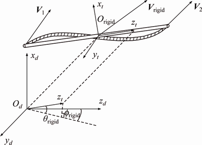
Figure 2 Schematic diagram of equivalent rigidization model
Expanding Eq. (22) using Eq. (23) and rearranging result in the equivalent Euler angles.
 (24)
(24)
The deformational velocity in the inertia reference frame Odxdydzd is given by
 (25)
(25)
Based on the kinetic characteristic of rigid body and using Figure 2, we find following relations:
 (26)
(26)
Expressing the velocity as the sum of their components with respect to the inertial reference frame and expanding Eq. (26) using them yield the components of angular velocity ��rigid with respect to the body frame:
 (27)
(27)
where

 (28)
(28)
So, the equivalent velocity Vrigid can be given by
 (29)
(29)
where Vo�� is the deformational velocity of barycenter, which can be obtained by
 (30)
(30)
Based on the law of conservation of mass and momentum, we can get the equivalent mass and the moment of inertia components:
 (31)
(31)
 (32)
(32)
So, a virtual rigid body, which owns similar dynamic characteristics to the original flexible suspension line, can be applied. Hereas, the modeling theory of multi-rigid-body system can be utilized to construct a unified dynamic model of flexible-rigid coupling multi-body system, the details of how to model and solve are as follows:
Step 1) Based on the equivalent rigidization model, a virtual rigid body can be constructed.
Step 2) Utilize modeling method of rigid multi-body system to construct a dynamic model
Step 3) Update the equivalent parameters of virtual rigid body.
Step 4) Solve dynamic equations to obtain the constraint forces
Step 5) Utilize the discrete solution for the kinetic characteristic of flexible body
Step 6) Go to Step 3.
Step 3 to Step 6 form an outer loop. Iterations at Step 5 are called inner iterations.
3 Modeling method of variable topology
3.1 Modeling process
A multi-body system in a topological non-tree is shown in Figure 3.
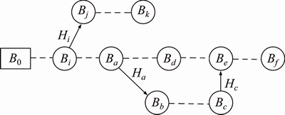
Figure 3 Topology of multi-body system
The original system can be divided into some subsystems by cutting off the joints of Ha, Hc, Hi, of which the result is shown in Figure 4. The cut-off joints can be replaced by constraint forces and moments RHab, RHce, RHij, which are shown in Figure 4. According to practical conditions, different joints can be selected for dividing system.
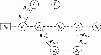
Figure 4 Topology after cutting off joints
Suitable modeling methods are selected to construct dynamic models of subsystems BjBk, B0Bf and BbBc, which are multi-body systems. If there is a flexible system, the equivalent rigidization model can be utilized firstly, and then suitable multi-rigid- body modeling method can be selected to continue modeling. Analyzing Ref. [21�C23] and Ref. [25, 27] which present a detail discussion of the modeling methods of vector mechanism, analytical mechanism, transfer matrix, and Kane method and rearranging result is the unified dynamic models for rigid multi-body systems:
 (33)
(33)
3.2 Iterative relations of constraint force
For holonomic constraints, the constraint equation can be given by
 (34)
(34)
where k is the number of cut-off joints; K is the total of joints; i, j are numbers of objects. The relationship between two objects and cut-off joint is that, Bi and Bj are two bodies interconnected by joints Hk, which point Bj.
Differentiation of Eq. (34) with respect to time in the inertial frame yields
 (35)
(35)
where
(l=i, j) (36)
 (37)
(37)
where s is the number of constraint equations of cut-off joint Hk.
For non-holonomic constraints, its constraint equation can be given by
 (38)
(38)
Differentiation of Eq. (38) with respect to time in the inertial frame yields
(39)
where

(l=i, j) (40)

(41)
Body i is assumed to belong to a subsystem, and the body j is assumed to belong to another one.
According to the joint location in the topology, we can get,
 (42)
(42)
where n is the total number of bodies; i and j are the numbers of adjoining bodies which are interconnected by cut-off joints. If l = 0 or n�Cl�C1=0, 06l��6 or 06(n-l-1)��6 will not exist.
Substituting constraint Eq. (35) or Eq. (39) into dynamic Eq. (33) and rearranging, we can get the iterative relation of constraint forces and moments.

 (43)
(43)
3.3 Solution algorithm
Considering multi-body system shown in Figure 3 and using iterative relation of constraint forces and moments result in constraint forces and moments RHab, RHce, RHij.

 (44)
(44)

 (45)
(45)
 (46)
(46)
According to modeling process, external force and moment of system R includes external forces and moments of all the bodies and constraint forces and moments among subsystems. It means that RHab includes RHce and RHij; RHce includes RHab and RHij; RHij includes RHab and RHce. CFA proposed in Ref. [15] can be utilized and the more details about the algorithm can be seen in Ref. [15]. The details of how to solve the iterative Eqs. (44)�C(46) are as follows.
Step 1) Set RHab=0. And according to the iterative relations, we can get array ��.
Step 2) Set each component of array RHab to be equal to one while the others are set to be equal to zero, respectively. And according to the iterative relations, we can get array ��.
Step 3) Base on the CFA, we can get RHab=�C���C1��.
Step 4) Substituting the expression of RHab, we can get the other constraint forces and moments.
4 Application examples
The dynamic model of internally carried air-launched system is taken as an example to verify the method above. The configuration of internally carried air-launched system is shown in Figure 5, where a parachute connects the payload by a riser, and the corresponding topology is depicted in the Figure 6, where the body B0 refers to carrier, body B1 refers to rocket, body B2 refers to flexible suspension line, body B3 refers to parachute treated as almost a rigid canopy. In Figure 5, there are four phases taken into account, the air launch preparation phase (Case=0), the rocket extraction phase (Case=1), the rocket rotation separation phase (Case=2) and the rocket in air movement phase (Case=3), which are more complicated to be simulated and their simulations have attracted many researchers. More details about air-launched phase can be seen in Ref. [7].

Figure 5 Air launch and its process
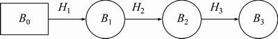
Figure 6 Topology of air-launched system
Firstly, we described the assumptions used to construct dynamic model for this system: 1) The potential energy on ground is zero. 2) The rocket goes along the slide rail with no lateral movements and the work of the friction is ignored. 3) During the air-launched process, the forces acting on the system include the gravity and aerodynamics forces. The details of how to model the entire air-launched process and the validation of numerical simulation are given below.
4.1 Aircraft dynamic model based on vector mechanisms
The kinetic equations of carrier aircraft [28], which can be divided into two equations, translation-kinetic equation and rotation-kinetic equation, can be derived from Newton��s Second Law of motion, which states that the summation of all external forces acting on a body must be equal to the time rate of change of its momentum, and the summation of all external moments acting on a body must be equal to the time rate of change of its angular momentum. Using Newton��s Second Law of motion and consulting Ref. [5] result in the translation-kinetic equation and rotation-kinetic equation.
 (47)
(47)
 (48)
(48)
where V0 is velocity vector in the inertia coordinate system; ��0 is angle velocity vector from motion coordinate system to earth coordinate system; F0 is external force of aircraft in the earth coordinate system; M0 is external moment of aircraft in body coordinate system.
And based on the Euler kinetic equation, relation between the angular velocity and the attitude represented as follows:
 (49)
(49)
where ��0x, ��0y, ��0z are projective values of angle velocity ��0 at body coordinate system; ��0, ��0, ��0 are attitude angles of aircraft; W0 is transformational matrix and expressed as
 (50)
(50)
4.2 Rocket-line-parachute system model based on Kane method
1) Generalized coordinates and virtual velocity
The position coordinates (x, y, z), attitude angles (��1, ��1, ��1) of aircraft, attitude angles (��2, ��2, ��2) of the suspension line, and attitude angles (��3, ��3, ��3) of the parachute are selected as the generalized coordinates. We used q and to denote the vector of the generalized coordinates and their derivative, respectively.
 (51)
(51)
 (52)
(52)
Consider the general condition, let��s define the vector arrays of the system virtual velocity in the global frame as v(vx, vy, vz), and the attitude angular velocity of aircraft, attitude angular velocity of the suspension line and attitude angular velocity of the parachute in each body local frame as: ��1(��1x, ��1y, ��1z), ��2(��2x, ��2y, ��2z) and ��3(��3x, ��3y, ��3z). The vector form of the virtual velocity are written as
 (53)
(53)
For simplifying writing, the virtual velocity can be rewritten as
 (54)
(54)
Based on the Euler kinetic equation, relation between the virtual velocity and the generalized velocity can be represented as follows:
 (55)
(55)
where

And the kinetic equation of the system can be given by
 (56)
(56)
2) Partial velocities
In the global frame, considering the virtual body i, i=1�C3, its velocity and angular velocity can be stated as follows:
 (57)
(57)
where V is the velocity of object��s barycenter in earth coordinate system; �� is angle velocity of object in its own body coordinate system; parameter of subscript 1 belongs to rocket; parameter of subscript 2 belongs to rope; parameter of subscript 3 belongs to parachute; Mij is the transformational matrix from i coordinate system to j coordinate system; subscript b in transformational matrix refers to body coordinate system; subscript g in transformational matrix refers to the earth coordinate system; L1 is a vector from front tiedown point to rocket��s barycenter in rocket��s body coordinate system; L21 is a vector from rope��s barycenter to front tiedown point in rope��s body coordinate system; L22 is a vector from back tiedown point to rope��s barycenter in rope��s body coordinate system; L3 is a vector from parachute��s barycenter to back tiedown point in parachute��s body coordinate system;  is the anti-symmetric matrix.
Based on Eq. (57) and the theory of Kane method, the partial velocities and the partial angular velocities of the body i, i=1�C3, are stated as follows:
 (58)
(58)
where

(59)
3) Generalized active force and generalized inertia force
The vector of generalized active force  of system can be expressed as
 (60)
(60)
where R is external force and moment and includes aerodynamic force and gravity.
 (61)
(61)
According to the theories of D`Alambert and Kane method, generalized inertia force can be expressed as
 (62)
(62)
where
 (63)
(63)
where A and B are both matrixes, which can be expressed as


where m is a mass matrix; J is the moment of inertia; and the meaning of subscript is the same as above.
4) Dynamic model
The Kane equation can be represented by
 (64)
(64)
Finally, substituting Eqs. (60)�C(63) into Kane Eq. (64) and considering kinetic Eq. (56), the simplest kinetic equation for this rocket-line- parachute system can be formulated:
 (65)
(65)
4.3 Airdrop system dynamic model for entire operation process
Considering the kinetic relations among the bodies in this system and the constraint form of cut-off joints, the constraint equations can be formulated:
 (66)
(66)
where

 (67)
(67)
where t0 is the setup time after air-launched stating; l0 is distance from rocket��s barycenter to tail part of cargo space; l10 is distance from top of rocket��s to tail of cargo space.
Based on Eq. (43), the iterative relations of constraint forces and moments in this system can be expressed as

(i=0, 1, 2) (68)
where i is the number of air-launched phase.
Above all, Eqs. (47)�C(49), Eqs. (65) and (68) compose the unified equations of motion for this system. And based on the equivalent rigidization model and the unified equations, we can get the kinetic characteristics of the system.
5 Verification model based on ADAMS
To verify the veracity of the theory and models in this paper, the corresponding verification model is built based on dynamic software ADAMS and 3D modeling software CATIA. Because it is not the focus of this paper, the modeling process is briefly described as follows and the details of how to model can be seen in Ref. [23].
A three-dimensional solid model is constructed, and then analyzed in CATIA in accordance with the design parameter for the carrier aircraft, the rocket, the suspension line and the parachute. The model is then imported into ADAMS to add quality attributes. Figure 7 shows three views of the air-launched system solid model. Physical modeling is done mainly in ADAMS, which allows for the expression of mechanical values. This is done through the addition of Kinematical constraints, driving constraints, forces, and moments to the solid model in ADAMS. As a result, relative motions and drives among the components are defined and given mechanical prosperities.
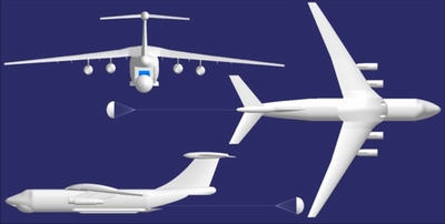
Figure 7 Three-dimensional solid model of air-launched system
5.1 Veracity of equivalent rigidization model
Simulation of opening parachute process is simulated first based on the equivalent rigidization model. We divide suspension line into sixty elements. The result is shown in Figure 8. We get the phenomenon of fishhook by numerical simulation, which is the same as the other researchers. So, the equivalent rigidization model in this paper is feasible and valid.
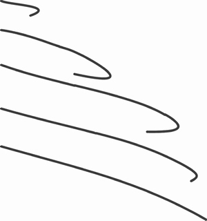
Figure 8 Phenomenon of fishhook
5.2 Veracity of dynamic modeling method of variable topology
The mathematical models are simulated at the same conditions to verify the feasibility and validity of the theory and models in this paper. The initial conditions of simulation are as follows. Initial altitude of aircraft is 10 km. Initial velocity of aircraft is 0.65 Mach. The weight of clear aircraft is 89000 kg. In the body frame, the moments of inertia of aircraft at axis x, y and z are respectively 540740 kg��m2, 737480 kg��m2, 117030 kg��m2. The area of wing is 300 m2. The length of wing is 51 m, the average chord is 6 m, the mass of rocket is 28000 kg. In the body frame, the moments of inertia of rocket at axis x, y and z are respectively 7870 kg��m2, 545000 kg��m2, 545000 kg��m2. The length of rocket is 18.5 m. The friction coefficient is 0.005. The characteristic drag of parachute is 10 m2. The length of flexible suspension line is 60 m. The mass of parachute is 1.798 kg. The trimming angle of attack is 1.2174��. The curves of the key parameters are shown in Figures 9�C11. In these Figures, line without explanation refers to results obtained by method in this paper and dashed line with explanation of VP refers to the results obtained by method of ADAMS.
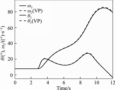
Figure 9 Curves of pitch angle and pitch angular velocity
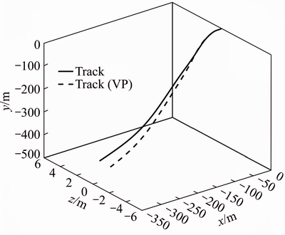
Figure 10 Curves of three-dimension track
Figure 9 shows pitch angle and pitch angular velocity in vertical plane. Figure 10 shows three-dimension track. Figure 11 shows two- dimension track. The simulation results show that pitch angle at about 3 s starts increasing, while air- launched process goes into the third step. At about 4 s, rocket separates from aircraft, while air- launched process goes into last step. And at about 10.5 s, the pitch angle is close to 90��, which is the largest one and whose angular velocity is equal to zero, and the time is suitable for rocket��s firing up. The simulation closely resembles the real condition. According to the comparison of the results, the dynamic responses of the two models are basically the same and the error ranges are under allowing. In conclusion, the theory and models in this paper are feasible and valid.

Figure 11 Curves of two-dimension track
6 Conclusions
The modeling method for rigid-flexible coupling multi-body system with variable topology based on the equivalent rigidization model, CFA and so on, has been presented. Considering the modeling process, solution algorithm and the air-launched examples, it can be seen that the modeling method has more advantages.
1) There is not any second derivative of generalized coordinates with respect to time in Eqs. (44)�C(46), which indicates that the equations of constraint forces and moments can be solved independently from equations of state variable. In addition, Eqs. (44)�C(46) are algebra equations. So, the method simplifies calculations, reduces the number of differential-algebraic equations, and increases the solving speed.
2) Dynamic models of different subsystems can be independently constructed from each other.
3) Considering that any constraints can be replaced by corresponding constraint forces and moments, the method is suitable for multi-body dynamic system with variable topology to construct the unified models.
4) Based on the method, design of control law can be easier.
5) Because the whole system is divided into some independent subsystems, performance of appointed bodies can be obtained more easily, and the analytical efficiency is increased.
References
[1] KE Peng, YAN Chun-xin, YANG Xue-song. Extraction phase simulation of cargo airdrop system [J]. Chinese Journal of Aeronautics, 2006, 19(4): 315�C321. DOI: 10.1016/S1000-9361(11)60334-8.
[2] CHEN Jie, SHI Zhong-ke. Aircraft modeling and simulation with cargo moving inside [J]. Chinese Journal of Aeronautics, 2009, 22(2): 191�C197. DOI: 10.1016/S1000-9361(08)60086- 2.
[3] YAN Chun-xin, KE Peng. Development and validation of the multi-body simulation software for the heavy cargo airdrop system [C]// 19th AIAA Aerodynamic Decelerator Systems Technology Conference and Seminar. Williamsburg, VA, AIAA 2007-2572. DOI: 10.2514/6.2007-2572.
[4] DESABRAIS K J, RILEY J, SADECK J, LEE C. Low-cost high-altitude low-opening cargo airdrop systems [J]. Journal of Aircraft, 2012, 49(1): 349�C354. DOI: 10.2514/1.C031527.
[5] CHEN Jie, MA Cun-bao, DONG Song. Kinetic characteristics analysis of aircraft during heavy cargo airdrop [J]. International Journal of Automation and Computing, 2014, 11(3): 313�C319. DOI: 10.1007/s11633-014-0794-5.
[6] LI Chun, TENG Hai-shan, ZHU Yan-hua, JIANG Wan-song, ZHOU Peng, HUANG Wei, CHEN Xu, LIU Jing-lei. Design and simulation for large parafoil fix line object homing algorithm [J]. Journal of Central South University, 2016, 23(9): 2276-2283. DOI: 10.1007/s11771-016-3285-8.
[7] SARIGUL-KLIJN M, SARIGUL-KLIJN N, HUDSON G C, HOLDER L, FRITZ D, COLONEL L. Flight testing of a gravity air launch method to enable responsive space access [C]// AIAA Space 2007 Conference & Exposition. Long Beach, California, 2007, AIAA 2007-6146. DOI: 10.2514/ 6.2007-6146.
[8] SARIGUL-KLIJN M, SARIGUL-KLIJN N, HUDSON G C, HOLDER L, LIESMAN G, SHELL D. Gravity air launching of earth-to-orbit space vehicles [C]// Space 2006. San Jose, California, AIAA 2006-7256. DOI: 10.2514/6.2006-7256.
[9] BONACETO B, STALKER P. Design and development of a new cargo parachute and container delivery system [C]// 18th AIAA Aerodynamic Decelerator Systems Technology Conference and Seminar. AIAA 2005-1647. DOI: 10.2514/ 6.2005-1647.
[10] WOLF D. Dynamic stability of a non-rigid parachute and payload system [J]. Journal of Aircraft, 1971, 8(8): 607�C609. DOI: 10.2514/3.59145.
[11] SARIGUL-KLIJN M, SARIGUL-KLIJN N, HUDSON G C, MCKINNRY B, MENZEL L, GRABOW E. Trade studies for air launching a small launch vehicle from a cargo aircraft [C]// 43rd AIAA Aerospace Sciences Meeting and Exhibit. Reno, Nevada, 2005, AIAA 2005-621. DOI: 10.2514/6.2005- 621
[12] HUDSON G C. Quick-reach responsive launch system [C]// 4th Responsive Space Conference. AIAA-RS4 2006-2003. DOI: 10.2514/6.2006-2003.
[13] SARIGULKLIGN N, SATIGULKLIGN M, NOEL C. Air-Launching earth to orbit: Effects of launch conditions and vehicle aerodynamics [J]. Journal of Spacecraft and Rockets, 2005, 42(3): 569�C572. DOI: 10.2514/1.8634.
[14] NOGUCHI Y, ARIME T, MATSUDA S, FUJI T, KANAYAMA H, DEPASQUALE D. Japanese air launch system concept and test plan [C]// Aerodynamic Decelerator Systems Technology Conferences. Daytona Beach, Florida, 2013, AIAA 2013-1331. DOI: 10.2514/6.2013-1331.
[15] ZHANG Qing-bin, QIAN Tang-gang, PENG Yong, WANG Hai-tao. Dynamics of parachute-capsule recovery system: Chaps. 3 [M]. Beijing: National Defense Industry Press, 2013: 30. (in Chinese)
[16] FULLER J D, TOLSON R H, RAISZADEH B. Multibody parachute flight simulations using singular perturbation theory [C]// 20th AIAA Aerodynamic Decelerator Systems Technology Conference and Seminar. Seattle, Washington, 2009, AIAA 2009-2920. DOI: 10.2514/6.2009-2920.
[17] ROMERO L M, RAY E S. Application of statistically derived CPAS parachute parameters [C]// Aerodynamic Decelerator Systems Technology Conferences & AIAA Aerodynamic Decelerator Systems (ADS) Conference. Daytona Beach, Florida, 2013, AIAA 2013-1266. DOI: 10. 2514/6.2013-1266.
[18] WU Gen-yong, HE Xing-suo, FRANK PAI P. Numerical and experimental investigation of nonlinear dynamics of highly flexible multibody systems [C]// 52nd AIAA/ASME/ASCE/AHS/ASC Structures, Structural Dynamics and Materials Conference. Denver, Colorado, 2011, AIAA 2011-1870. DOI: 10.2514/6.2011-1870.
[19] DESABRAIS K J. Aerodynamic forces on an airdrop platform [C]// 18th AIAA Aerodynamic Decelerator Systems Technology Conference and Seminar. AIAA 2005-1634. DOI: 10.2514/6.2005-1634.
[20] ZHANG Qing-bin. A new parachute deployment model by multibody dynamics [C]// 17th AIAA Aerodynamic Decelerator Systems Technology Conference and Seminar. Monterey, California, AIAA 2003-2134. DOI: 10.2514/ 6.2003-2134.
[21] ZHANG Xiang, HUANG Yi-yong, CHEN Xiao-qian, HAN Wei. Modeling of a space flexible probe-cone docking system based on the Kane method [J]. Chinese Journal of Aeronautics, 2014, 27(2): 248�C258. DOI: 10.1016/j.cja.2014. 02.020.
[22] ZHOU Chun-lin, WANG Bo-xing, LI Jing-lan, XIONG Rong. Dynamic modeling of a wave glider [J]. Frontiers of Information Technology & Electronic Engineering, 2017, 18(9): 1295�C1304. DOI: 10.1631/FITEE.1700294.
[23] ZHANG Jiu-xing, XU Hao-jun, ZHANG Deng-cheng, LIU Dong-liang. Safety modeling and simulation of multi-factor coupling heavy-equipment airdrop [J]. Chinese Journal of Aeronautics, 2014, 27(7): 1062�C1069. DOI: 10.1016/j.cja. 2014.08.014.
[24] DRAGOLJUB V, OLGICA L, VOJISLAV B. Development of dynamic-mathematical model of hydraulic excavator [J]. Journal of Central South University, 2017, 24(9): 2010�C2018. DOI: https://doi.org/10.1007/s11771-017-3610-x.
[25] DOHERR K F, SCHILLING H. Nine-degree-of-freedom simulation of rotating parachute systems [J]. Journal of Aircraft, 1992, 29(5): 774�C781. DOI: 10.2514/3.46245.
[26] KANG B S, SHYY Y K. Design of flexible bodies in multibody dynamic systems using equivalent static load method [C]// 49th AIAA/ASME/ASCE/AHS/ASC Structures, Structural Dynamics, and Materials Conference. Schaumburg, IL, 2008, AIAA2008-1708. DOI: 10.2514/6. 2008-1708.
[27] RUI Xiao-ting, YUN Lai-feng, LU Yu-qi, WANG Guo-ping. Transfer matrix method of multibody system and its applications Chaps. 1, 7 [M]. Beijing: Science Press, 2008. (in Chinese)
[28] ZHENG Wu-ji, LI Ying-hui, QU Liang, YUAN Guo-qiang. Dynamic envelope determination based on differential manifold theory [J]. Journal of Aircraft, 2017, 54(5): 2005�C2009. DOI: 10.2514/1.C034258.
(Edited by YANG Hua)
���ĵ���
��װʽ���з������ػ���Ķ���ѧģ��
ժҪ�������������װʽ���з������ϵͳ����װ��Ͷϵͳ�ı����˽ṹ��-����϶���ϵͳ��Ϊ������ʽͳһ�Ķ���ѧģ�ͣ������ⵥһ��ģ���������ཨģ���̣�������ڵ�Ч�ջ��Ľ�ģ�������ڽ�ģ�����У��ض���ϵͳ�������������˽ṹ�����仯�Ľ¡��������������ϵͳ���õ�Ч�ջ��Ľ�ģ������������ϵͳ�ɸ�����Ҫѡ����ʵĽ�ģ�������ڼ�������У�����Լ���������㷨��ʸ����ѧ���ۿɽ�Լ������״̬���̶�����⡣����װʽ���з���ϵͳ�Ķ���ѧģ�ͽ���Ϊ���ӣ���֤�˻��ڵ�Ч�ջ��Ľ�ģ��������Ч�Ժ���ȷ�ԣ����ֽν����˿��з���ϵͳ�Ķ���ѧģ�͡���������ģ������ȣ��������۵õ��Ķ���ѧģ���ڲ�ͬ�ξ���ͳһ����ʽ����ģ���̼��ҳ�����Ч�ջ��Ľ�ģ��������������ۿ�Ӧ�������Ƶĸ�-����϶���ϵͳ��
�ؼ��ʣ�������ϣ������˽ṹ����װʽ���з������ػ��������ϵͳ����������
Received date: 2017-06-17; Accepted date: 2018-02-28
Corresponding author: ZHENG Wu-ji, PhD Candidate; Tel: +86-15339171508; E-mail: 18729228764@163.com; ORCID: 0000-0002- 0365-5454
Abstract: For rigid-flexible coupling multi-body with variable topology, such as the system of internally carried air-launched or heavy cargo airdrop, in order to construct a dynamic model with unified form, avoid redundancy in the modeling process and make the solution independent, a method based on the equivalent rigidization model was proposed. It divides a system into independent subsystems by cutting off the joints, of which types are changed with the operation process of the system. And models of different subsystems can be constructed via selecting suitable modeling methods. Subsystem models with flexible bodies are on the basis of the equivalent rigidization model which replaces the flexible bodies with the virtual rigid bodies. And the solution for sanction, which is based on the constraints force algorithm (CFA) and vector mechanics, can be independent on the state equations. The internally carried air-launched system was taken as an example for verifying validity and feasibility of the method and theory. The dynamic model of aircraft-rocket-parachute system in the entire phase was constructed. Comparing the modeling method with the others, the modeling process was programmed; and form of the model is unified and simple. The model, method and theory can be used to analyze other similar systems such as heavy cargo airdrop system and capsule parachute recovery system.
