J. Cent. South Univ. Technol. (2010) 17: 991-999

DOI: 10.1007/s11771-010-0589-y

Node scattering manipulation based on trajectory model in wireless sensor network

PEI Zhi-qiang(裴智强), XU Chang-qing(徐昌庆), TENG Jin(藤劲)

Department of Electronic Engineering, Shanghai Jiaotong University, Shanghai 200240, China

? Central South University  Press and Springer-Verlag Berlin Heidelberg 2010

Key words:

wireless sensor network; node scattering manipulation; trajectory model; energy consumption；

1 Introduction

In recent years, much attention has been paid to the development of wireless sensor network (WSN), and many schemes have been presented [1-5]. They are classified into three categories: selecting active nodes intentionally [6-8], adjusting node transmitting power [2-3] and adopting mobile nodes [9-14].

Due to the network redundancy, only a part of sensor nodes are in the active state to save energy. KUMAR et al [6], ZOU and CHAKRABARTY [7], and WANG et al [8] discussed this problem, resolved the difficulty to select active nodes, and reached the following conclusions: determining the quantity of sensors required by WSN, ensuring the least sensors in the active state and guaranteeing the coverage and connectivity degree. In practice, the network topology needs to be controlled or adjusted [1-3], which is very suitable for the environment without the ability of attachment. For instance, LI et al [2] proposed a cone- based distributed topology control algorithm and proved that letting α(α is the degree of cone around one node) be equal to 5π/6 by adjusting transmitting power of nodes was a critical condition to guarantee the network connectivity.

After mobile sensors are adopted, the network topology in WSN can be automatically optimized. All of the proposed schemes or algorithms can be classed into the distributed [9, 11] and the center-controlled [10, 12-13]. The former is that every node exchanges information with its connected neighbors and determines its final position, independently. The later is that base station collects information from sensors, such as their ID and positions, and determines the final position of every sensor, to which these sensors would be relocated.

The previous achievements only focused on the following two aspects: the selection of optimal topology and the method to relocate sensor nodes by using mobile nodes. However, it has never mentioned the method to scatter nodes from aircraft. Resolving this problem is very practical and significant in many applications because the process of scattering nodes is prerequisite.

It is well known that energy is a key issue in WSN. All the efforts should be focused on decreasing energy consumption. In previous works, the extra energy had to be consumed in order to improve the coverage and connectivity, which were the key objectives of WSN, that is, the previous achievements were at the price of node energy. It would be a creative innovation, while all or part of energy, consumed by sensors during their relocation, was replaced by that of other devices. Therefore, a scheme, named node scattering manipulation, was proposed to resolve the above problem. The following two aspects presented the basic idea of this scheme: first, during node scattering, the initial states of every sensor, including the velocity and direction, were manipulated so that it could land in a region with a certain probability; then, every sensor node was relocated in order to improve the coverage and connectivity. Our scheme receives the following virtues:

(1) Practical. It is easy to realize our scheme in practice.

(2) Saving energy. The reason is that all or part of energy, consumed by sensors during node relocation, is replaced by that of scattering device.

(3) Improving coverage. This will be expatiated in section 4.

(4) Approximate ideal topology. Every sensor is near to its ideal position after landing on the ground.

Whichever deployment scheme is adopted, it is unavoidable that sensors randomly land on the ground and that the coverage holes must exist. This problem belongs to inter-discipline. It is necessary to study the trajectory model and stochastic distribution of sensors falling on the ground. Obviously, many uncertain factors have a significant impact on sensors during their descent. But, in this work, only the following factors are considered: gravity, wind force and air resistance. Among them, gravity is a constant, because it is related to sensor weight, and the others are regarded as stochastic variables.

It was necessary to point out that, in this work, only one node was scattered every time. Obviously, this was not efficient, and was also not suitable for the applications, under which a cluster of sensors were scattered every time. Thus, in the future, we will study the scheme.

2 Preliminaries

2.1 Notations throughout this work

 and  The ideal and actual positions of one sensor. and are their coordinates, respectively.

p_p: The position of a flying plane while one sensor is cast. (p_px, p_py, p_pz) are its coordinates.

p_s(t): The position of one sensor at time t during its descent. (p_sx(t), p_sy(t), p_sz(t)) are its coordinates.

v_s(t): The velocity of a sensor at time t during its descent. Its initial velocity v_s(0) is equal to v_p+v_ss, where v_p is the velocity of a flying plane, and v_ss is the relative velocity of one sensor to v_p at t=0.

In this work, the units of all kinds of variables are as follows: length, m; velocity, m/s; time, s; mass, kg; acceleration, m/s²; force, N; influence factors k_w and k_ar, N?s/m; area, m².

2.2 Assumptions on sensors and network configuration

(1) All sensors can accurately obtain their own location via certain localization techniques, such as GPS (global positioning system) or positioning algorithms.

(2) All sensors have the same configuration. In other words, they have the same transmitting and sensing ranges, computation capability, storage memory, available energy etc.

(3) All sensors have the limited movement capability, i.e., they can adjust their own positions like the schemes in Ref.[13]. The maximum movement distance is D_m.

(4) All sensors have the same shape and mass. Without loss of generality, let m be a constant which represents the mass of every sensor.

(5) The area of interest is supposed to be a 2-D plane. To be consistent with 3-D space, a point in the monitored area is also described as 3-D vector p=(p_x, p_y, p_z), where p_z is the constant.

(6) Every sensor can transmit its data packets without collisions via certain medium access control protocols.

2.3 Projectile motion

The motion trajectory of a projectile has been studied in physics. Without loss of generality, the expression

                             (1)

denotes the position of one sensor falling on the ground. This model does not take other factors into consideration except for the gravitation. Here, it is easy to receive the following formulas:

                         (2)

                         (3)

In practice, it is difficult to know the accurate landing positions of air-borne sensors, because there are many uncertain factors, among which the air turbulence, more commonly called the wind force, and air resistance play a major part. So, it is necessary to study the impacts of wind force and air resistance on projectile motion during sensor descent.

2.4 Impact of wind force on projectile motion

According to physics, wind has a significant influence on a falling object. It is difficult to accurately describe this influence. However, in this work, an influence factor, k_w, is defined to describe it.

A model is first established to demonstrate the wind. Though the wind often changes its direction and  intensity, yet it still can be considered to be relatively stable and constant during the flying period of a dropping node. So, it is supposed that the parameters of wind, namely, bearing and intensity here, are random and independent among different air-borne sensors, and are unchanged during the descent of one air-borne sensor node.

Suppose that the wind velocity, v_w, would be a vector parallel to the level ground surface. Without loss of generality, v_w=(v_wx, v_wy, v_wz), where v_wz is equal to zero. v_w can be also expressed as another 3-D vector under the polar coordinate system: v_w=(v_w, θ, φ), where v_w=|v_w|,   0≤θ≤2π, and φ=π/2 because of v_wz=0.

To describe the randomness of v_w, define two random variables, v_w and θ. Their distribution was uniform over the interval [v₁, v₂] and [θ₁, θ₂], respectively.

A force, F_w, can be initiated on a projectile object while the wind acts on this object. Here, F_w can be written as:

F_w=k_wv_w, k_w＞0                              (4)

While a falling object is influenced by only two forces: the gravity and wind force, F_w will be changed depending on different values of k_w, that is, one sensor node will land on different positions, as shown in Fig.1. Here, the following parameters are adopted. m=0.5 kg, v_s(0)=(10 m/s, 0 m/s, 0 m/s), |v_w|=20 m/s, θ=π/3, and p_p=(0 m, 0 m, 100 m).

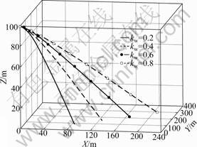
Fig.1 Impact of wind on projectile object

2.5 Impact of air resistance on projectile motion

Air resistance, F_ar, is significantly influenced by many factors, such as the shape and velocity of a falling object. Here, a model is established to demonstrate the impact of air resistance. The shape of a falling object is supposed to be globose, and its impact on air resistance can be regarded as a constant. The velocity of a falling object also has significant impact on air resistance during the descent of this object. Without loss of generality, let k_ar be a factor to describe the influences of air resistance, thus, F_ar is written as:

F_ar=-k_arv_s                                   (5)

Different results of F_ar, depending on different values of k_ar, are shown in Fig.2. Here, the following parameters are adopted: m=0.5 kg, v_s(0)=(10 m/s, 0 m/s, 0 m/s) and p_p=(0 m, 0 m, 100 m).

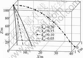
Fig.2 Impact of air resistance on projectile object

2.6 Trajectory of projectile motion

One sensor is significantly influenced by many factors during its descent. In this work, other factors are ignored except for the gravity, wind force and air resistance. It is not so unreasonable to posit that the force, F(t), acted on a sensor, is the sum of all the forces compelled on the sensor. Therefore, F(t) is written as:

F(t)=F_w+F_ar+G=k_wv_w-k_arv_s(t)+G                 (6)

According to the physics, p_s(t), defined in section 2.1, can be written as:

           (7)

3 Node deployment scheme

In previous achievements, the network topology was optimized by manpower deployment or by sensor relocation. In this work, a scheme, named node scattering manipulation, was designed to deploy sensors over the area of interest. This scheme can reduce the energy consumption during node relocation. Simultaneously, a trajectory model was proposed to describe the descent of one sensor.

3.1 Scattering manipulation of sensor nodes

The process of scattering sensors is shown in Fig.3. While one sensor is thrown out of a plane, it is initialized with velocity v_ss, and it falls on the ground according to the projectile motion trajectory. The launching device, like a pistol, can be adopted to drive a sensor flying. The

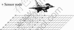
Fig.3 Scattering process of sensors by plane

driving force is not from powder, but from gases at high pressure. In order to improve the deployment efficiency, multiple sensors can be cast at a time, which will be studied in the future.

According to formulas (1)-(3), it is easy to calculate the ideal landing position of every sensor. The initial position and velocity of a flying plane are p_p and v_p, respectively, and those of one air-born node are also p_p and v_s, respectively. Therefore, the ideal position of one air-born node falling on the ground is expressed as:

                           (8)

wherep_py+

 and  . In particular, F_x, F_y and F_z are the components of F(t), i.e., F(t)=(F_x, F_y, F_z).

3.2 Landing point

The landing deviation from desired position for each sensor can now be expressed by the superposition of two stochastic processes, namely, the passive deviation driven by wind force and original deviation complying with a normal distribution.

First, the random variable, v_w, is analyzed. It has been mentioned that v_w and θ are two random variables with uniform distribution over the interval [v₁, v₂] and [θ₁, θ₂], respectively. Let f_pd(?) be the probability density function of the relevant variable. According to probability and statistics for engineers, the probability density functions f_pd(v_wx) and f_pd(v_wy) in 3-D right-angle coordinate system can be deduced as Eqs.(9) and (10), respectively:

         (9)

where 

;

and

        (10)

where  and C_vwy2=C_vw?

Then, the velocity of a sensor at time t during its descent is analyzed. v_s(t) is deduced as follows:

               (11)

where  C_vsy=C_vsv_wy+ v_sy(0) and

The falling process of one sensor is analyzed. Let T be the time of one sensor landing on the ground from aircraft. According to physics, position p_s(T), on which one sensor lands, is deduced as:

                      (12)

Substituting Eq.(11) into Eq.(12), p_s(T) is optimized as:

                  (13)

where C_px=p_px-   and  

Next, we analyze f_pd(p_sx(T)) and f_pd(p_sy(T)) of point p_s(T), on which one sensor node lands under the impacts of wind, air resistance and gravity. Because f_pd(v_wx) and f_pd(v_wy) are obtained, it is very easy to deduce the probability density function of p_s(T) as follows:

        (14)

where ≤≤ and ≤≤

At last, we analyze the probability density function of  under the superposition of two independent random variables, namely, the passive deviation driven by all impact factors and the original deviation complying with a normal distribution N(μ, σ), where μ(=(μ_x, μ_y)) and σ(=(σ_x, σ_y)) are the mean value and standard deviation of N(μ, σ), respectively. It is further supposed that μ_x and μ_y are independent, so do σ_x and σ_y. Without loss of generality, let f_pd(p_nrpx) and f_pd(p_nrpx) be the probability density functions of N(μ, σ) along x and y axis components, respectively, which indicate the random distribution of position of one sensor landing on the ground only considering the original deviation. Formally, f_pd(p_nrpx) and f_pd(p_nrpx) can be written as:

      (15)

Thus, the distributions of the position of one sensor node falling on the ground with all the impacts can be written as:

                                     (16)

Their distribution curves are shown in Fig.4. The following parameters are adopted: v₁=2 m/s, v₂=4 m/s, θ₁=π/6, θ₂=π/3, μ=(0 m, 0 m), σ=(10 m, 10 m), m=0.5 kg,

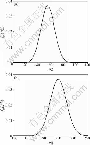
Fig.4 Curves of(a) and(b)

g=9.8 m²/s, k_ar=0.05 N?s/m, k_w=0.4 N?s/m, p_p=(0 m, 0 m, 100 m) and v_s=(10 m/s, 0 m/s, 0 m/s).

It is necessary to point out that the above two density distributions are deduced for single and independent node. Sensors in a batch, however, are not independent, because they undergo the same wind turbulence, which will be studied in the future. One more thing to say is that, the above model for wind is simplified to easily understand. Actually, the wind velocity vector is a 3-D vector instead of a 2-D one. So, there is a vertical component. In this work, falling time T is also a random variable influenced by that vertical wind speed. And to take this component into consideration, some other processing methods, mainly another integral, are required.

3.3 Sensor relocation

Once sensors are scattered, not all of them lie on their own ideal positions. Some sensors must be relocated to approach ideal deployment pattern. Here, a simple relocation scheme is applied. Its principle is that one sensor moves from its landing point to its ideal target position, and that its movement distance is d. The mobility of a sensor is limited, and its maximum movement distance is D_m [13]. One sensor is incapable of moving to its ideal target position while d＞D_m, which leads to non-full-coverage or non-connectivity. The following lemma is proposed to study the coverage percentage.

Lemma 1 If and only if the probability of s lying in , p(s, ), is not less than P, the requirement of applications is satisfied after sensor relocation, where P is the coverage percentage required by some applications, and  is a disc of radius D_m centered at.

Proof It is assumed that M nodes are deployed over the target area. Let M₁ be the number of nodes that lie in their own disc.

If According to the statistics principle, the following expression always holds:

.

This expression indicates that M₁ of M sensors land in their own disc. The coverage percentage is M₁/M after sensor relocation, which approaches to p(s, ) while M→∞. Because p(s, )≥P, the requirement of applications is satisfied after sensor relocation.

Only if Because the requirement of application is satisfied after sensor relocation, at least MP nodes land in their own disc, . Due to M₁Z⁺ and MP≤M₁, the following expression always holds:

Therefore,  p(s, )≥P.

4 Simulation

In order to evaluate the performance of the scheme, the simulation was conducted using MATLAB language. The ideal deployment patterns in Refs.[15-16] were adopted, and the monitored target area was supposed to be 500 m×10 000 m. The main objectives are that sensors are forced to land as close to their own ideal position as possible, and that node energy consumption is decreased to great extent during node relocation.

In this section, metrics, which are the measurements of the proposed deployment scheme, are first stated. Then, the impacts of all kinds of factors on the deployment scheme are introduced and analyzed. Next, the cost is quantified. At last, two results, which are realized by the scheme and by that in Ref.[13], are compared.

4.1 Metrics

Let A_R be the total area of the target region of interest, and let A_CR be the area of region covered by sensors. The efficient coverage of WSN is defined as E_C. Formally, E_C is written as: E_C=A_CR/A_R.

Let C_IR be the coverage improvement of the monitored area. In order to easily analyze the performance of the deployment scheme, C_IR is defined as:

, where  and  are areas of

regions covered by sensors after and before sensor relocation, respectively.

Let C_s be the cost of all sensors during their relocation. Without loss of generality, the value of C_s is defined as the sum of the movement distance of every sensor.

At last, it must be pointed out that the scattering device deploys only one sensor node at a time.

4.2 Effective coverage of WSN

The target area is fully covered while all the sensor nodes lie on their ideal positions. In practice, it is difficult for us to achieve this object. Therefore, node relocation scheme is adopted. Fig.5 describes the effective coverage performance of our deployment scheme. It is necessary to point out that E_C≤, and here, this is explained. Because the distance of two connected neighboring sensors is 2r_s instead of  or other values in Refs.[8, 15-16], thus, the following

expression always holds: E_C≤

, where l and w are the length and width of the target area, respectively.

While the value of σ is unchanged, which decides the concentrated degree of node distribution, E_C is approximately stable before node relocation. The reason is that σ is consistent while WSN is deployed repetitively. However, E_C increases with the increase of D_m after node relocation, because more sensors are relocated to their ideal positions, as shown in Fig.5(a).

While the value of D_m is unchanged, E_C continuously decreases with the increase of σ before node relocation, because the node distribution is sparser, i.e. more regions are not covered by any sensors. After sensors are relocated, E_C is improved largely. For instance, E_C is improved by about 30% at D_m=50 and σ=(15, 15). Here, this is explained. Sensors are close to their ideal positions while the value of σ is small, i.e., almost all of them can be relocated to their own ideal positions due to p(s, )→1. Therefore, E_C can be improved to upper limit  However, due to the limited movement distance, more sensors lose the capability of being relocated to their ideal positions while the value of σ is gradually increased, i.e., E_C is smaller than upper limit and has the descending tendency with the increase of σ, as shown in Fig.5(b).

4.3 Impact of all kinds of factors on E_C

The impacts of D_m and σ on E_C have been analyzed in section 4.2, here, those of k_ar and k_w on E_C are investigated.

As shown in Fig.6(a), E_C gradually decreases with the increase of k_ar, which results from the following reasons. According to formula (5), the variation of k_ar will result in the change of F_AR. Thus, k_ar has a significant impact on the landing point of one sensor. As shown in Fig.2, sensors are further away from their ideal positions while the value of k_ar is larger, i.e., the node distribution is sparse and uneven with the increase of k_ar.

There is the same explanation for the impact of k_w on E_C (Fig.6(b)).

4.4 Costs of plane or sensors

Obviously, the curve tendency of C_s is increasing at initial stage, and finally, it is stable, while all variables are increasing, as shown in Fig.7. The reason is that more cost must be paid to improve the coverage, and that the effective coverage is approximate to upper limit

In order to test the performance of this deployment scheme, we provide the comparison between our scheme and that in Ref.[13], as shown in Fig.8. Obviously, this deployment scheme improves the coverage percentage extremely and deduces the deployment cost greatly while the value of D_m is larger.

5 Conclusions and future work

(1) An effective deployment scheme, named node scattering manipulation based on trajectory modeling, is proposed to deploy sensors. This scheme ensures that every sensor lands on the ground as near to its ideal position as possible, decreases the energy consumption during its relocation, saves the total energy of network, and improves the network characteristics. In practice, this scheme is operable and can be realized easily. Simulation results demonstrate the superiority of this deployment scheme.

(2) Only one sensor is thrown out of a plane at a time. This scattering method is of low efficiency and not suitable for the WSN application of massive sensors, although it can provide the theoretical foundation for

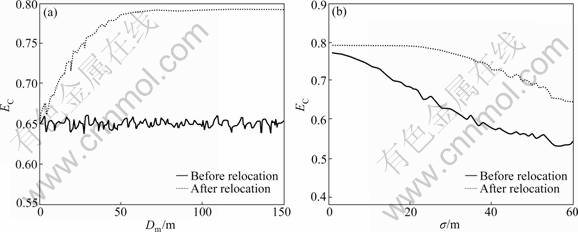
Fig.5 Efficient coverage of WSN: (a) σ=(15 m, 15 m); (b) D_m=50 m

Fig.6 Impacts of k_ar and k_w on E_C: (a) D_m=50 m, σ=(15 m, 15 m), k_w=0.4 N?s/m; (b) D_m=50 m, σ=(15 m, 15 m), k_ar=0.05 N?s/m

Fig.7 Impacts of D_m, k_ar, k_w and σ on C_s: (a) σ=(15 m, 15 m), k_ar=0.05 N?s/m, k_w=0.4 N?s/m; (b) D_m=50 m, σ=(15 m, 15 m), k_w=   0.4 N?s/m; (c) D_m=50 m, σ=(15 m, 15 m), k_ar=0.05 N?s/m; (d) D_m=50 m, k_ar=0.05 N?s/m, k_w=0.4 N?s/m

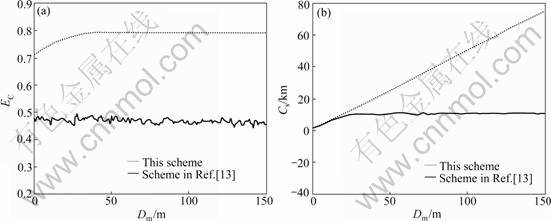
Fig.8 Comparison between this scheme and scheme in Ref.[13]: (a) E_C vs D_m; (b) C_s vs D_m

studying node deployment. Thus, in the future work, we will study the deployment scheme, which can scatter multiple sensors or a cluster of sensors at a time, and further study the trajectory modeling during the descent of multiple sensors.

References

[1] HOWARD A, MATARI? M J,SUKHATME G S. An incremental self-deployment algorithm for mobile sensor network [J]. Autonomous Robots: Special Issue on Intelligent Embedded Systems, 2002, 13(2): 113-126.

[2] LI L, HALPERN J Y, BAHL P, WANG Y M, WATTENHOFER R. Analysis of a cone-based distributed topology control algorithm for wireless multi-hop networks [C]// Proceedings of ACM Symposium on Principles of Distributed Computing. Newport, Rhode Island, 2001: 264-273.

[3] LI N, HOY J C, SHA L. Design and analysis of an MST-based topology control algorithm [J]. IEEE Transactions on Wireless Communications, 2005, 4(3): 1195-1206.

[4] TAN Chang-geng, XU Ke, WANG Jian-xin, CHEN Song-qiao. A sink moving scheme based on local residual energy of nodes in wireless sensor networks [J]. Journal of Central South University of Technology, 2009, 16(2): 265-268.

[5] MA C L, INOUE A, ZHANG T. Ultrahigh performance of Ti-based glassy alloy tube sensor for Coriolis mass flowmeter [J]. Transactions of Nonferrous Metals Society of China, 2006, 16(s): s202-s205.

[6] KUMAR S, LAI T H, BALOGH J. On k-coverage in a mostly sleeping sensor network [J]. Wireless Networks, 2008, 14(3): 144- 158.

[7] ZOU Y, CHAKRABARTY K. A distributed coverage- and connectivity-centric technique for selecting active nodes in wireless sensor networks [J]. IEEE Transactions on Computers, 2005, 54(8): 978-991.

[8] WANG X R, XING G L, ZHANG Y F, LU C Y, PLESS R, GILL C. Integrated coverage and connectivity configuration in wireless sensor networks [C]// Proceedings of the 1st International Conference on Embedded Networked Sensor Systems. Los Angeles, 2003: 28-39.

[9] WANG G L, CAO G H, la PORTA T. Movement-assisted sensor deployment [J]. IEEE Transactions on Mobile Computing, 2006, 5(6): 2469-2479.

[10] WU Jie, YANG Shu-hui. Smart: A scan-based movement-assisted deployment method in wireless sensor networks [C]// The 24th Annual Joint Conference of IEEE Computer and Communications Societies. Miami, 2005: 2313-2324.

[11] ZOU Y, CHAKRABARTY K. Sensor deployment and target localization based on virtual forces [C]// The 22nd Annual Joint Conference of the IEEE Computer and Communications Societies. San Francisco, 2003: 1293-1303.

[12] WANG G L, CAO G H, la PORTA T, ZHANG W S. Sensor relocation in mobile sensor networks [C]// The 24th Annual Joint Conference of the IEEE Computer and Communications Societies. Miami, 2005: 2302-2312.

[13] CHELLAPPAN S, BAI X L, MA B, XUAN D, XU C Q. Mobility limited flip-based sensor network deployment [J]. IEEE Transactions on Parallel and Distributed Systems, 2007, 18(2): 199-211.

[14] HOWARD A, MATARIC M J, SUKHATME G S. Mobile sensor network deployment using potential fields: A distributed, scalable solution to the area coverage problem [C]// Proceedings of the 6th International Symposium on Distributed Autonomous Robotics Systems. Fukuoka, 2002: 299-308.

[15] KUMAR S, LAI T H, ARORA A. Barrier coverage with wireless sensors [C]// Proceedings of the 11th Annual International Conference on Mobile Computing and Networking. Cologne, 2005: 284-298.

[16] BAI X L, KUMAR S, XUAN D, YUN Z Q, LAI T H. Deploying wireless sensors to achieve both coverage and connectivity [C]// Proceedings of the 7th ACM International Symposium on Mobile Ad Hoc Networking and Computing (Mobihoc). Florence, 2006: 131- 142.

(Edited by YANG You-ping)

Foundation item: Project(2007AA01Z224) supported by National High-Tech Research and Development Program of China

Received date: 2009-11-13; Accepted date: 2010-03-25

Corresponding author: PEI Zhi-qiang, Doctoral candidate; Tel: +86-21-34204344; E-mail: pzqsjtu@sjtu.edu.cn; pzqjlu@sohu.com