
J. Cent. South Univ. Technol. (2008) 15: 860-868
DOI: 10.1007/s11771-008-0158-9![]()
Swarm intelligence based dynamic obstacle avoidance for mobile robots under unknown environment using WSN
XUE Han(Ѧ ��), MA Hong-xu(������)
(College of Electromechanical Engineering and Automation, National University of Defense Technology,
Changsha 410073, China)
Abstract:
To solve dynamic obstacle avoidance problems, a novel algorithm was put forward with the advantages of wireless sensor network (WSN). In view of moving velocity and direction of both the obstacles and robots, a mathematic model was built based on the exposure model, exposure direction and critical speeds of sensors. Ant colony optimization (ACO) algorithm based on bionic swarm intelligence was used for solution of the multi-objective optimization. Energy consumption and topology of the WSN were also discussed. A practical implementation with real WSN and real mobile robots were carried out. In environment with multiple obstacles, the convergence curve of the shortest path length shows that as iterative generation grows, the length of the shortest path decreases and finally reaches a stable and optimal value. Comparisons show that using sensor information fusion can greatly improve the accuracy in comparison with single sensor. The successful path of robots without collision validates the efficiency, stability and accuracy of the proposed algorithm, which is proved to be better than tradition genetic algorithm (GA) for dynamic obstacle avoidance in real time.
Key words:
1 Introduction
WSN is a novel network technique integrating modern wireless communication, micro sensor and computer network, which has extensive prospects and high application value in defence, environment supervision, household automation, transportation and many other fields[1-3]. WSN comprises of different types of sensor nodes that co-operatively perform tasks like collaborative sensing, environment monitoring, etc.
Most current path planning methods largely computed offline are unsuitable for application to a real-time scenario with dynamic moving obstacles, which is different from priori environment amongst static obstacles[4-6]. Dynamic obstacle avoidance is an exciting research field and hot topic of mobile robots, with its close link to sensor design, data fusion, map building, localization, off-line optimized path planning methods and navigation methods. A number of solutions have been proposed in the literature to dynamic obstacle avoidance problems. Most of the earliest obstacle avoidance methods were based on the potential field approach. There have been many other approaches that have departed from the potential field approach. The vector field histogram (VFH) method proposed by BORENSTEIN and KOREN[7] transformed a local map into a one-dimensional discretized ��polar obstacle density�� function. FOX et al[8] searched a space of the robot��s translational and rotational velocities. The TerraScout project at Carnegie Mellon University incorporated FAJEN and WARREN��s original model into their obstacle avoidance system. While potential fields are still used for dynamic obstacle avoidance, there are a number of other commonly used techniques. The formulation of behaviors for autonomous agents is studied using the dynamical systems approach to behavior. SCH?NER et al[9] described a framework for designing behaviors for autonomous robots. FAJEN et al[10-11] devised a model of human navigation based upon experiments with human subjects. Subjects walking straight towards a goal were presented with an obstacle located at different initial angles and distances. In this case, angular acceleration away from the obstacle decreased with the increase of both obstacle angle and distance.
As a novel and developing evolutionary algorithm, swarm intelligence has become a hotspot of the domain of artificial intelligence in recent years[12-15]. There exists a special relationship between swarm intelligence and artificial life. Completed theory and application research have shown that swarm intelligence is effective in solving most global random optimization problems. Swarm intelligence has provided complicated and distributed strategies for traditional structure optimization problems and so far has obtained fine success in many fields. Through analysing multiple constraints and utilizing the autonomy and mutation of swarm intelligence, the ant colony algorithm based on swarm intelligence was used for dynamic obstacle avoidance problems.
In this work, utilizing the advantages of WSN, a novel dynamic obstacle avoidance algorithm for mobile robots based on ant colony optimization using swarm intelligence was proposed. By enhancing the entire performance, a new choice of moving obstacle avoidance for mobile robots was provided, which meets the real-time demand under unknown environment. The energy consumption and topology of WSN were also discussed.
2 M and behaviour definition
The global coordinate system which shows the position relationship between the moving obstacle and robot is built, as shown in Fig.1, where the velocity of the robot is denoted by vR; the velocity of the obstacle is denoted by vO; the relative velocity of the robot to the obstacle is denoted by ?v; the component of ?v along the direction from the robot to the obstacle is denoted by vl; the component of ?v vertical to the direction from the robot to the obstacle is denoted by v��; the angle of the robot is denoted by symbol ��; the angle of the obstacle is denoted by ��; the angle of direction from the robot to the obstacle is denoted by ��; the angle of direction from ��v to vl is denoted by ��. The relationship among these variables can be expressed as follows:
vl=vRcos (��-��)-vOcos (��-��) (1)
v��=vRsin (��-��)-vOsin (��-��) (2)
![]() (3)
(3)

1Collision model between robot and obstacle
Through computation, Eqn.(4) can be obtained as:
![]()
(4)
Then Eqn.(4) can be rewritten as
![]()
(5)
Since ��v, vR and vO form a triangle, according to the sine rule and cosine rule, Eqn.(6) can be obtained as follows:
![]() (6)
(6)
![]() (7)
(7)
![]() (8)
(8)
Therefore, Eqn.(5) can be simplified as
![]() (9)
(9)
Then the remaining work is to work out the best solutions (��vR, ����) for energy, time and other optimal performance goals. The space coordinate system is shown in Fig.2. The zonal region between two lines is the collision region. In order to avoid collision, robot should select the space which is out of the zonal region and leave the collision region as quickly as possible.

Fig.2 Safe zonal region in space coordinate system
The test environment is the working office in the laboratory. The size of the test robot is 0.32 m��0.24 m�� 0.28 m, while the obstacles are the moving vehicles that are smaller than the robots.
3 Sensor model and critical speed
3.1 Sensor model
According to the type and capability of sensors, a sensor model is a function from the environment state to a set of measurement readings. The environment is mainly constituted of obstacles and the positions and orientations of robots. For the occupancy representation, a probabilistic model of a sensor is required to relate different possible measurements to the configuration of the environment. When measuring the distance between sensors and obstacles, the distance detected from the sensor may not accurately reflect the true distance due to various reasons such as corruption by noises and calibration errors. The probabilistic sensor model, therefore, is needed to reflect these uncertainties into the distance detection. The sensor model is shown in Fig.3.

3Sof robot detecting distance
The sensors are not able to detect signals when the intensity of signals is weaker than that of noises. Meanwhile, each sensor has its maximal measuring range. Assuming that Fmin is the minimal effective measured value of a sensor and Fmax is the maximal measured value. The signal intensity at position p of the detected target measured by sensor s satisfies:
Fmin��S(s, p)��Fmax (10)
The model of the sensor is:
 (11)
(11)
where d(s, p) is the Euclidean distance between the sensor s and target p; �� and k are parameters depending on sensor technique, �� is the calibration of the sensor and K is the decaying rate of signals. Eqn.(11) indicates that sensing ability of sensors decreases with the increase of distance between sensors and targets in an exponential way.
3.2 Exposure model and exposure direction
The concept of exposure describes the exposure degree of the moving obstacles in sensor network. If the exposure of an obstacle in given time is larger than the threshold value of a sensor, the sensor can discover the moving obstacle. In some cases, exposure value only depends on the distance between sensors and obstacles, and the moving time of obstacles. Exposure model in the energy form is expressed as Eqn.(12), which is the integral of signal intensity detected by the sensor:
![]() (12)
(12)
Define the direction from sensor to the obstacle is the least exposure direction (LED), and the direction from the obstacle to the sensor is the maximal exposure direction (BED), as shown in Fig.4. It has been proved that sensors obtain minimal exposure value when obstacles move along LED, while sensors obtain maximal exposure value when obstacles move along BED.

4Diagram of BED and LED
3.3 Critical speeds
From Eqn.(11), the distance from which sensors can detect effectively is computed as:
d(s, p)��![]() (13)
(13)
When the velocity of obstacles is zero, sensors obtain the maximal exposure value:
![]() (14)
(14)
When Et����T, sensor network cannot detect the obstacle. So it is desired that:
Et�ܦ�T (15)
Given the threshold Et, when the exposure value of obstacles under maximal exposure model is equal to Et, the corresponding velocity is the immeasurably critical speed, which satisfies Eqn.(16):
 (16)
(16)
where vc is the critical speed.
When k=2, the critical speed can be computed as
![]() (17)
(17)
4 WSN and robot system
4.1 WSN and robots
Although WSN is a novel network technique, the data processing ability and executive power of WSN are quite limited, and strict constraint on energy is one of its significant restrictions. Mobile robot can automatically deploy and calibrate sensors, detect and dispose the errors and irrational deployment of the sensors, make dynamic response to the hardware or environment changes, enable distributed WSN systems to work well continually in longer time and improve the stability of the entire system. As smart action performers, mobile robots can recharge sensors, thus greatly improving the adaptability and maneuverability of mobile nodes and enabling the nodes to be freely deployed in environment without charging establishment.
Meanwhile, mobile robots have powerful computing ability and great mobility, but the deficiency on perception ability limits the development of its intelligence. WSN provides mobile robots with the real-time global perception to monitor continuous and long-rage environment and search optimal path as a medium of communication and computation. Therefore, robots equipped with WSN system make the two systems cooperate with each other, enhance the perception ability of mobile robots and improve environment control ability of WSN.
4.2 Sensor networks architecture
The module of sensor nodes is shown in Fig.5. Each of these scattered sensor nodes has the capabilities in collecting data and transmitting data back to the sink and the end users. Data are routed back to the end user by a multihop infrastructure through the sink, which may communicate with the task manager node via Internet or Satellite.
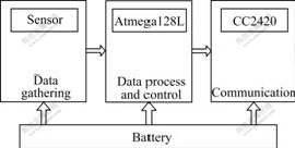
Fig.5 Sensor node module
The protocol stack used by the sink and all sensor nodes is given in Fig.6. This protocol stack combines power and routing awareness, integrates data with networking protocols, communicates power efficiently through the wireless medium, and promotes cooperative efforts of sensor nodes. The protocol stack consists of the application layer, transport layer, network layer, data link layer, physical layer, power management plane, mobility management plane, and task management plane. Depending on the sensing tasks, different types of application software can be built and used on the application layer.

Fig.6 Sensor networks protocol stack
4.3 Map update based on sensor fusion
The required environment information for mobile robots in path planning under unknown dynamic environment is collected from sensors. Due to nondeterministic errors, environment influence, communication time delay and transmission mistake, it is difficult for single sensor to guarantee the accuracy and reliability of input information and exact description of working environments. The grid occupancy information from multiple sensors is redundant, complementary, real-time and low-cost, which enable robots to update maps in the process of continuous environment detection and effectively reduce sensor errors and incorrect readings for quick and parallel analysis of field environment.
With wireless sensor network, mobile robots detect and collect local environment information in real-time mode, frequently regulate paths and re-plan according to new environment information. Mobile robots maintain global map of environment and plan path according to their current map. Then they forward along the path for a while. During this period, they update global map based on new information collected, and re-plan or regulate existing paths following the updated global map. They continue the loop mentioned above until they reach the target position.
Histogrammic in motion mapping, Bayesian approach[16], Kalman filter, Dempster-Shafer theory and fuzzy logic algorithm[17] are four standard multi-sensor fusion approaches applied to path planning of mobile robots. The Bayesian model was used in this work. The updated occupancy probability is determined using the Bayesian conditional probability theory according to the distance from the grid to the sensor. The Bayesian model supports a theoretical basis for the probability map.
![]()
![]() i, respectivelySi��{1, 0} i (Si=0) (Si=0) The probability of occupancy of grid i is as follows:
i, respectivelySi��{1, 0} i (Si=0) (Si=0) The probability of occupancy of grid i is as follows:
![]() (18)
(18)
By the B rule, Si
 (19)
(19)
 (20)
(20)
Eqns.(19) and (20) is
![]() (21)
(21)
![]() (22)
(22)
Eqn.(22)
![]() (23)
(23)
where
![]() (24)
(24)
![]() (25)
(25)
Ci ri-1 ri
![]() (26)
(26)
t Ci
![]()
![]() (27)
(27)
4.4 Energy consumption analysis
The WSN is subjected to a certain set of resource constraints such as limited on-board battery power and network communication bandwidth. Clustering has been well received as an effective way to reduce the energy consumption of WSN. Clustering is defined as the process of choosing a subset of wireless sensor nodes as cluster heads for a given WSN. Therefore, data traffic generated at each sensor node can be routed via cluster heads to the network sink. Clustering can enhance the energy efficiency in many aspects and has been widely used in sensor hierarchical routing and topology control. Cluster heads receive and forward the traffic originated by cluster members to the network sink. Clustering is also used for data aggregation and fusion. Cluster heads aggregate and fuse the information collected at the cluster members, making the overall network traffic significantly reduced. Thus, the energy efficiency will be greatly enhanced.
In the single hop communication scheme where several sensor nodes of the same type distribute in a circular cluster domain, the role of cluster-head sensor node is acted by each sensor node in turn. Energy consumption is computed as follows:
![]() (28)
(28)
where N is the number of data transmitted in a period; r is the radius of the cluster; l is the energy consumption of transmission circuit; c is the transmission cost exponent and �� is the fixed factor of transmission cost.
In the multi-hop scheme, the number of relay data packet of each sensor node in the nth circle is:
![]() (29)
(29)
where R is the thickness of each circle in the multi-hop scheme. Each sensor node in the nth circle not only relays the cn data packet, but also transmits its own data packet. In each period with N data transmitted, the energy consumption is:
![]() (30)
(30)
Sensor nodes in the first lever consume the most amount of energy:
![]() (31)
(31)
In the case of R=a, Eqn.(31) is simplified to the same as single hop scheme which costs the least energy.
The multi-hop network is partitioned and the cluster-heads chosen with four stages are shown in Fig.7. For example, given the system topology of sensor network, the neighbourhood relation is represented by the links connecting nodes in Fig.7(a). In Fig.7(b), the part of multi-hop network is partitioned into five clusters. The identification of a cluster-head denotes which cluster it belongs to. In the choosing stage, each cluster decides its new head according to the remaining battery power.

Fig.7 Cluster-heads chosen with four stages: (a) Tree stage; (b) Partitioning stage; (c) Choosing stage; (d) Hierarchy clustering stage
Fig.7(c) shows the change of these clusters while others remain the same. Finally, these cluster-heads constitute a higher-level cluster in Fig.7(d).
5 Algorithm based on swarm intelligence5.1 Ant colony optimization algorithm
Ant colony algorithm is a novel heuristic evolutionary optimization algorithm proposed by Italian scholar DORIGO in 1991[18-20]. It mimics ant behaviors in nature and has the characteristics of distributed computing, positive feedback of information and heuristic search[21]. Ant colony algorithm is rendered suitable for a variety of widespread applications in multiple combinatorial optimization problems, not only in discrete systems but also in continuous systems, such as scheduling, quadratic assignment, network rooting, etc.
The frame of multiple constrained optimization solution based on ant colony algorithm is as follows.
Ant Colony Algorithm
Input: Weighted graph, neighborhood into.
While: Termination not met do
Compute-initial pheromone, node dist potential Schedule activities
Ant based solution construction
Pheromone update
Node distance potential update
End activities
Update and record the best solution in the population
Output: Best, candidate to optimal solution
5.2 ACO algorithm for robot obstacle avoidance
Using ACO algorithm described above, the optimal solutions (?vR, ?��) for energy, time and other optimal performance goals are worked out. When the robot points to the moving obstacle, it should adjust its direction. To drive the robot to reach the goal as quickly as possible, the direction of the robot and the line from the robot to its goal, that is ����+��, should be minimum. Meanwhile, the faster the speed of the robot, the better performance of collision avoidance. The obstacle avoidance function can be represented as follows:
f(��vR, ����)=w1|��vR|+w2|��+����| (32)
The procedures of optimal algorithm are listed as follows.
Step 1 System initialization: initialize the time, iterative time and pheromone. Place m ants on each initial position.
Step 2 Selection: the transition probability of ant k from position i to position j at time t is given by
 (33)
(33)
where ��i, j(t) is the reciprocal of objective function; �� is the influencing weight of ��i, j(t) to the whole transition probability; �� is the influencing weight of ��i, j(t) to the whole transition probability; and ![]() is the set of positions connected with node i and not visited by ant k.
is the set of positions connected with node i and not visited by ant k.
Step 3 Compute the objective functions of each ant and record the current optimal solution of the problem.
Step 4 Update the local pheromone and the concentration of pheromone. Update locally the pheromone of the chosen parameter as follows:
![]() (34)
(34)
where �� is the volatile factor of pheromone of the parameter, 0���ѣ�1.
Step 5 Record optimal solutions. The pheromone is updated globally as follows:
![]() (35)
(35)
where a1 is a constant.
Step 6 Check the termination condition: if the cycle index is less than preset times or the optimization target is not reached, go to Step 2).
Step 7 Output the optimal solution and terminate the procedure.
6 Experimental results
6.1 Hardware configuration and results
The algorithm was implemented on real mobile nodes. The main components on the top layer were MICAz sensor nodes composed of MCU, ATMega128L, and the wireless communication chip, CC2420. A sensor board could be connected with MICAz additionally. The top layer was assigned to getting the sensing data and communicate with other nodes, informing bottom layer with serial ports. The WSN built could work well for a long time.
Table 1 Sensor node speification

The algorithm was tested under dynamic environ- ment with moving environment as shown in Fig.8, where the squares represent the robot and the circles represent moving objects. The results show that the robot can go from the initial position to the destination without colliding with any dynamic obstacle.

Fig.8 Moving states under dynamic environment with moving obstacles: (a) Initial state; (b) Moving state 1; (c) Moving state 2; (d) Moving state 3; (e) Moving state 4; (f) Final state
The comparison between genetic algorithm and ant colony optimization algorithm on the time robots spend in obstacle avoidance and the length of path robots walk is listed in Table 2. The computer equipment is Pentium 4 CPU 1.4GHz. Through the efficient and useful algorithm, the optimal path can soon be computed. The results show that the method based on ant colony optimization algorithm is superior to the genetic algorithm.
Table 2 Performance comparison between GA and ACO

6.2 Effect of iterative times on length of shortest path
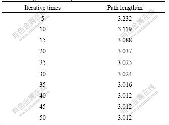
The length of shortest path after different iterative times is shown in Table 3. It can be seen that as iterative times grow, the length of shortest path decreases. It reaches 3.012 after 40 times of iteration.
Table 3 Length of shortest path after different iterative times
6.3 Effect of WSN on measurement error
The measurement accuracy of single sensor and information fusion based on WSN was compared. Fig.9 shows the comparison results on distance errors of the two methods. The result shows that using sensor information fusion can greatly improve the accuracy in comparison with single sensor.
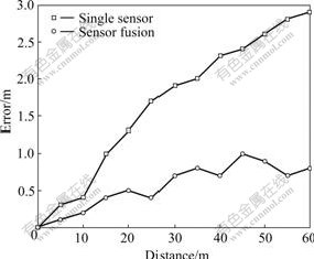
Fig.9 Error comparison between single sensor and information fusion based on WSN
7 Conclusions1) A novel dynamic obstacle avoidance algorithm is proposed utilizing the advantages of WSN. A practical implementation with real WSN and real mobile robots are carried out. Results show that using sensor information fusion can greatly improve the accuracy in comparison with using single sensor.
2) Ant colony algorithm based on bionic swarm intelligence is integrated. The convergence curve of the shortest path length shows the convergence of the algorithm. The algorithm is proved to enhance the entire performance of tradition genetic algorithm under real-time environment with multiple dynamic obstacles.
3) As a novel approach for real-time dynamic obstacle avoidance, the algorithm promotes the cooperation between mobile robots and WSN.
References
[1] GRACANIN D. A service-centric modeI for wireless sensor networks [J]. IEEE Journal on Selected Areas in Communications��2005, 23(6): 1159-1166.
[2] AKYILDIZ I F, SU W, SANKARASUBRAMANIAM Y, CAYIRCI E. Wireless sensor networks: A survey [J]. Computer Networks, 2002, 38(4): 393-422.
[3] BRAGINSKY D, ESTRIN D. Rumor routing algorithm for sensor networks [C]// Proceedings of the 1st Workshop on Sensor Networks and Applications. Atlanta: ACM Press, 2002: 22-31.
[4] KHATIB O. Real-time obstacle avoidance for manipulators and mobile robots [J]. Journal of Robotics Research, 1986, 5(1): 90-98.
[5] OGREN P, LEONARD N E. A convergent dynamic window approach to obstacle avoidance [J]. IEEE Trans on Robotics and Automation, 2005, 21(2): 188-195.
[6] TANG Ping, ZHANG Qi, YANG Yi-min. Studying on path planning and dynamic obstacle avoiding of soccer robot [C]// Proceedings of the 3rd World Congress on Intelligent Control and Automation. Discataway IEEE, 2000: 1244-1247. (in Chinese)
[7] BORENSTEIN J, KOREN Y. The vector field histogram-fast obstacle avoidance for mobile robots [J]. IEEE Transactions on Robotics and Automation, 1991, 7(3): 278-288.
[8] FOX D, BURGARD W, THRUN S. The dynamic window approach to collision avoidance [J]. IEEE Robotics & Automation Magazine, 1997, 4(1): 23-33.
[9] SCH?NER G, DOSEM, ENGELS C. Dynamics of behavior: Theory and applications for autonomous robot architectures [J]. Robotics and Autonomous Systems, 1995, 16(1): 213-245.
[10] FAJEN B R, WARREN W H. Behavioral dynamics of steering, obstacle avoidance, and route selection [J]. Journal of Experimental Psychology: Human Perception and Performance, 2003, 29(2): 343-362.
[11] FAJEN B R, WARREN W H, TERMIZER S, KAEBLING L P. A dynamical model of steering, obstacle avoidance, and route selection [J]. International Journal of Computer Vision, 2003, 54(1/2): 13-34.
[12] SCHMICKL T, THENIUS R, CRAILSHEIM K. Simulating swarm intelligence in honey bees: Foraging in differently fluctuating environments [C]// GECCO 2005 - Genetic and Evolutionary Computation Conference. New York: Association for Computing Machinery, 2005: 273-274.
[13] KENNEDY J, EBERHART R C. Swarm Intelligence [M]. San Francisco: Morgan Kaufmann, 2001.
[14] BONABEAU E, DORIGO M, THERAULAZ G. Swarm intelligence: From natural to artificial systems [M]. New York: Oxford University Press, 1999.
[15] LIU H B, ABRAHAM A, CLERC M. Chaotic dynamic characteristics in swarm intelligence [J]. Applied Soft Computing, 2007, 7(3): 1019-1026.
[16] ELFES A. Using occupancy grids for mobile robot perception and navigation [J]. Computer, 1989, 22(6): 249-265.
[17] RUSSO F, RAMPONI G. Fuzzy methods for multi-sensor data fusion [J]. IEEE Trans on Instrum Meas, 1994, 43(2): 288-291.
[18] COLORNI A, DORIGO M, MANIEZZO V. Distributed optimization by ant colonies [C]// Proc First European Conference on Artificial Life. Cambridge:MIT Press,1992: 134-142.
[19] DORIGO M, MANIEZZO V, COLORNI A. The ant system: optimization by a colony of cooperating agents [J]. IEEE Transactions on Systems, Man, and Cybernetics, Part B, 1996, 26(1): 29-41.
[20] DORIGO M, GAMBARDELLAL M. Ant colony system: A cooperative learning approach to the traveling salesman problem [J]. IEEE Transaction on Evolutionary Computation, 1997, 1(1): 53-66.
[21] DORIGO M, DI CARO G, GAMBARDELLA L M. Ant algorithms for discrete optimization [J]. Artificial Life, 1999, 5(2): 137-172.
Foundation item: Project(60475035) supported by the National Natural Science Foundation of China
Received date: 2008-03-29; Accepted date: 2008-05-11
Corresponding author: XUE Han, PhD; Tel: +86-13467555439; E-mail: xdjs@163.com
(Edited by ZHAO Jun)
Abstract: To solve dynamic obstacle avoidance problems, a novel algorithm was put forward with the advantages of wireless sensor network (WSN). In view of moving velocity and direction of both the obstacles and robots, a mathematic model was built based on the exposure model, exposure direction and critical speeds of sensors. Ant colony optimization (ACO) algorithm based on bionic swarm intelligence was used for solution of the multi-objective optimization. Energy consumption and topology of the WSN were also discussed. A practical implementation with real WSN and real mobile robots were carried out. In environment with multiple obstacles, the convergence curve of the shortest path length shows that as iterative generation grows, the length of the shortest path decreases and finally reaches a stable and optimal value. Comparisons show that using sensor information fusion can greatly improve the accuracy in comparison with single sensor. The successful path of robots without collision validates the efficiency, stability and accuracy of the proposed algorithm, which is proved to be better than tradition genetic algorithm (GA) for dynamic obstacle avoidance in real time.
