
J. Cent. South Univ. Technol. (2010) 17: 406-412
DOI: 10.1007/s11771-010-0060-0 ![]()
Optimization of support vector machine power load forecasting model based on data mining and Lyapunov exponents
NIU Dong-xiao(ţ����), WANG Yong-li(������), MA Xiao-yong(��С��)
School of Economics and Management, North China Electric Power University, Beijing 102206, China
? Central South University Press and Springer-Verlag Berlin Heidelberg 2010
Abstract:
According to the chaotic and non-linear characters of power load data, the time series matrix is established with the theory of phase-space reconstruction, and then Lyapunov exponents with chaotic time series are computed to determine the time delay and the embedding dimension. Due to different features of the data, data mining algorithm is conducted to classify the data into different groups. Redundant information is eliminated by the advantage of data mining technology, and the historical loads that have highly similar features with the forecasting day are searched by the system. As a result, the training data can be decreased and the computing speed can also be improved when constructing support vector machine (SVM) model. Then, SVM algorithm is used to predict power load with parameters that get in pretreatment. In order to prove the effectiveness of the new model, the calculation with data mining SVM algorithm is compared with that of single SVM and back propagation network. It can be seen that the new DSVM algorithm effectively improves the forecast accuracy by 0.75%, 1.10% and 1.73% compared with SVM for two random dimensions of 11-dimension, 14-dimension and BP network, respectively. This indicates that the DSVM gains perfect improvement effect in the short-term power load forecasting.
Key words:
1 Introduction
During recent decades, numerous investigations have been carried out to improve the accuracy of electricity load forecasting. One method is to forecast future electricity load considering weather factors in the historical load data. Generally, it is known as the Box-Jenkins autoregressive integrated moving average (ARIMA). CHRISTIANSE [1] and PARK et al [2] designed exponential smoothing models by Fourier series transformation for electricity load forecasting. Hence, many researchers took related factors into account, such as seasonal temperature and day type [3-4]. MBAMALU and EL-HAWARY [5] proposed multiplicative autoregressive(AR) models that considered seasonal factors in load forecasting. DOUGLAS et al [6] considered verifying the impacts of temperature on the forecasting model. SADOWNIK and BARBOSA [7] proposed dynamic nonlinear models for load forecasting.
Chaos refers to the phenomenon, similar to a random, which comes forth in the certainty system without rules. Chaotic time series exists in many natural economic phenomena such as the price change in stock market [8] and some other economic chaos [9]. According to the chaotic solution with stochastic nature in the inherent certainty of nonlinear systems, it is predictable in the short term but unpredictable in the long term. At present chaotic time series forecasting methods include global prediction [10], and forecast method based on Lyapunov exponents [11]. In local forecast method based on the dynamic theory, the forecast is very suitable for chaotic time series, which is better than the global prediction. The result of neural network prediction is similar to that of the local forecast method [12]. The commonly used methods are mainly adding-weight one-rank local-region method and the method based on the largest Lyapunov exponent.
Support vector machine (SVM) implements the structural risk minimization principle rather than the empirical risk minimization principle implemented by most of the traditional neural network models. Many scholars have researched it [13-17].
In the last 20 years, chaotic theory and statistic learning theory have become mature frequently and the use of load prediction has become more and more popular. According to the characters of chaotic time series, the SVM prediction model based on Lyapunov exponents and data mining was established in this work, which combined the phase space delay coordinate reconstruction theory, and different groups were divided according to different features by data mining technology. And then, the optimizing SVM theory was used to verify its effectiveness in short-term power load forecasting of some electric networks.
2 Chaotic time series and Lyapunov exponents
According to chaos theory [18-19], the driving factors influenced each other in chaotic system. Therefore, the digital points obtained according to time are relative. At present, people have proposed the phase space delay coordinate reconstruction method to analyze the factors of serial dynamics. In the system, generally, the dimension is very great and even infinite in the phase space, and the dimension cannot be known in many situations. In fact, the phase space delay coordinate reconstruction method can expand the given time series x1, x2, ��, xn-1, xn, �� to three-dimensional space and even higher, so the information that is exposed sufficiently from time series can be classified and extracted.
The technology of reconstruction phase space is the premise to calculate Lyapunov exponents. In electric power system, actual loading series of single argument {x(ti)=1, 2, 3, ��, n} can be obtained with gap ?t. The structural character of system attractors is included in this time series. The specific method that can estimate the information of phase space reconstruction in single argument time series is as follows:
In this method, the time series can be calculated to m-dimensional phase space. The time delay is ��=k?t (k= 1, 2, ��). In previous permutation, every column makes up a phase point of m-dimensional phase space, and each phase point has ![]() components. These np=n-(m-1)�� phase points {x(tj), j=1, 2, ��, np} compose a fancies pattern in m-dimensional phase space, and the continuation of these phase points describes the evolutionary trace of system in the phase space.
components. These np=n-(m-1)�� phase points {x(tj), j=1, 2, ��, np} compose a fancies pattern in m-dimensional phase space, and the continuation of these phase points describes the evolutionary trace of system in the phase space.
The process of calculation of Lyapunov exponents and extraction of maximal Lyapunov exponent in single argument time series is as follows:
(1) Reconstructing m-dimensional phase space with time series.
(2) Choosing minimal �� that marks the correlation among phase spaces.
(3) In the continuation m-dimensional phase space, the initial phase point A(t1) is chosen as a reference point. There are m components in the phase space, which are x(t1), x(t1+��), x(t1+2��), ��, x[t1+(m-1)��].
3 Data mining preprocessing technology
3.1 Fuzzy classification disposing influencing factors
As to short load curve, weather is a very important influencing factor. It should be considered as influencing factor in order to improve the accuracy of short load forecasting. In order to obtain the relationship between weather factors and load swing, it needs to draw some chats and load swing, it needs to draw some chats of points. A conclusion can be drawn through these chats. The factors have more influence on loading and can be acquired from weather forecast containing daily highest temperature, daily lowest temperature, daily average temperature, daily rainfall and some other features.
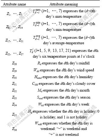
We select the typical (such as weekend or holiday), daily highest temperature, daily average temperature, daily lowest temperature, daily rainfall, daily wind speed and cloudy cover and daily seasonal attribute as random disturbance factors to short-term load. They can be seen in Table 1. Although the daily wind speed and cloudy cover cannot influence the load curve obviously, according to the above analysis, they have been chosen as the influential factors [20].
Table 1 Initial decision table
3.2 Selecting features with data mining
Data mining technology is a process of searching new relation, pattern and trend with pattern recognition technology, statistic and mathematic technology, which is to mine the information that has potential value. The functions can be implemented as follows.
(1) Classification. Build variant categories to describe things according to the attribute and character of the object. The category of the event can also be predicted. The sample data contain the data item of identification sample that belongs to a category.
(2) Clustering. Recognize intrinsic regulation of data analysis and classify the factors into variant categories according to these regulations.
(3) Association. Search for relative events or records, deduce the potential relations among the events, and recognize the pattern that may occur repeatedly. It can be collated according to correlation degree.
(4) Sequence pattern. Like association analysis, the correlation analysis on the relation among item sets can be expanded in a period of time, that is to say, the sequence pattern is related with time variable.
(5) Forecasting. Analyze the law of development of objects and forecast coming trend.
3.3 Selecting daily data based on gray relation analysis method for forecasting
3.3.1 Gray relation analysis theory
Relation analysis is a method that analyzes the extent of relation among factors in gray system theory, the essence can judge the extent of the factors according to the relation of caves. Detailed processes are as follows.
(1) Constructing sequence matrix. Analyze the relation taxis after the data classification bank is constructed. Hypothesizing that T0 represents the weather character of forecasting date, if the weather forecasting reports that the highest temperature is 40 ��, the average temperature is 25 ��, the lowest temperature is 15 ��, the rainfall is 20 mm, then T0=(T0(1), T0(2), T0(3), T0(4))=(40, 25, 15, 20). In this way, construct comparing sequence with daily weather data of the obtained data bank, which are represented as T1, T2, ��, Tn:
 (1)
(1)
(2) Nondimension. Process data with the method of initiation to eliminate dimension. The formulas are:
![]() (2)
(2)
Nondimension matrix is:
 (3)
(3)
(3) Calculating relation coefficient as follows:
![]()
 (4)
(4)
In this formula, i=0, 1, 2, ��, n; k=1, 2, ��, m, �� is resolution ratio, �ѡ�[0, 1], generally, ��=0.5. Then, the relation coefficient matrix can be obtained:
 (5)
(5)
(4) Calculating association degree as follows:
![]() i=1, 2, ��, n (6)
i=1, 2, ��, n (6)
3.3.2 Ascertain history loading sequence for forecasting
The reference sequence is the meteorologic factor index vector of forecasting data T0; and the comparing sequence is the meteorologic factor index vector of history data that are similar to the forecasting data in weather Tt. Then, calculate the associated degree between T0 and Tt, which is rt. Set a threshold value ��, and then choose these data whose correlation degree satisfies rt�ݦ�. At last, arrange these loading data orderly to be a new sequence.
4 SVM prediction model
The given time series {x1, x2, ��, xN} is separated into two parts. The previous ntr data are used as training sample to compute parameters values and the rest data as testing sample to prove the effectiveness of the model. The one-dimensional time series is converted into poly-dimensional matrix by reconstructing phase-space. Time delay is 1. The m-dimensional matrix is established as follows.
 ,
,  .
.
where X is the input matrix and Y is the output matrix. X and Y satisfy equation ��i, ��i*��0, and ��i* and ��i are relaxation factors. When the basic structure of the time series is determined, SVM can be used to train and predict the samples. The regression equation is
![]()
![]()
(7)
where ai and ai* are Lagrange multipliers with ai��ai*=0 and ai, ai*��0 for any i=1, 2, ��, l. Using Mercer��s theorem, the regression was obtained by solving a finite dimensional QP problem in the dual space. This can avoid explicit knowledge of the high dimensional mapping and the only use of the related kernel function.
The prediction model of the next time point is
 (8)
(8)
5 SVM based on Lyapunov exponents and data mining
The whole process of SVM based on Lyapunov exponents and data mining is shown in Fig.1.
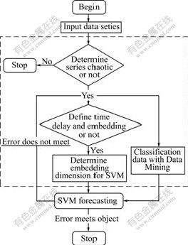
Fig.1 Calculation process of SVM forecasting model based on Lyapunov exponents and data mining
It can be seen that the calculation process includes the following five important steps.
Step 1: Establish a single-variable time series according to the historical power load data. Then, use Wolf method to determine whether the series is chaotic or not by computing Lyapunov exponents.
Step 2: Define time delay and work out the embedding dimension, then make data preprocessing. The embedding dimension and the number of phase points determined by Lyapunov method are used to restrict phase space.
Step 3: Input the history data and pre-process with the combination data mining technology that is introduced above, then the training and testing sample banks that have the most similar weather character could be got.
Step 4: Construct the needed history loading sequence C={C1, C2, ��, Cs} with gray relation analysis method, and divide the data based on data mining technology. There are s groups of weather forecasting data that contain the average temperature, the highest temperature, the lowest temperature and daily rainfall; D={d1, d2, ��, dn} is the daily weather data of n days before the forecasting date. Meanwhile, every factor di contains s groups of data.
Step 5: Establish the objective functions by using training sample. Then, convert previous functions into their dual problems, thus ai, ai* and b can be worked out. And then, they are substituted into Eq.(8). In this way, the predicted values of the subsequent time points can be worked out.
6 Application and analysis
Lyapunov exponents represent the average speed of scatter among neighborhoods in a system. A positive Lyapunov exponent weighs the segregation degree of average index number about two adjacent tracks, and a negative Lyapunov exponent judges the approach degree. If a discrete nonlinear system is dissipative, relatively stable and positive, Lyapunov exponent can be computed to judge whether the time series is chaotic or not [21].
According to the character of chaotic time series, the embedding dimension and Lyapunov exponents can be computed with the method. The dimensional value can be determined when the curve of Lyapunov exponents becomes stationary. Then, the embedding dimension and the time delay, which are the parameters of SVM model, can be calculated.
61 Choosing samples
Power load data in an area of Hebei Province,China, is used to prove the effectiveness of the model. The power load data from 0:00 on 3/25/2004 to 24:00 on 4/21/2006 are used as training sample to establish the single-variable time series {x(t1), x(t2), ��, x(t948)}. And the power load data from 1:00 to 24:00 on 4/23/2006 are used as testing sample.
In order to investigate the performance of the forecasting system thoroughly, the power system in Hebei Province, China, with different typical load characteristics and weather conditions are considered in this work. As a larger power supply system in China, Hebei Province satisfies the electrical needs of the north of China and the northeast of China. Fig.2 illustrates the quarter-by-quarter electricity demands of the system for more than two years in the area of Hebei Province, China.
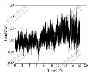
Fig.2 Distribution of power load in Hebei Province of China from 5/1/2004 to 5/28/2006
From Fig.2, the following common characteristics of the loads can be observed: the load series has multiple seasonal patterns, corresponding to a daily, weekly and monthly periodicity, respectively; the loads are also influenced by the calendar effect, i.e., weekend and holidays; sometimes, the demand presents high volatility and no constant means. From the observations above, it can be concluded that there are different regimes in the load series during different periods.
6.2 Data analysis
For the training sample, ��=1 is determined and Wolf method is used to compute Lyapunov exponents and embedding dimension. Firstly, The power load time series shows chaotic character due to �ˣ�0. Secondly, according to the theory, when the embedding dimension is 12, the Lyapunov exponent �� begins to show stable trend. Therefore, the embedding dimension is chosen as 12. The above parameters are used to reconstruct the phase-space. The results are shown in Table 2 and Fig.3.
Table 2��Relationship between embedding dimension (m) and Lyapunov exponent (��)
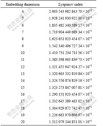
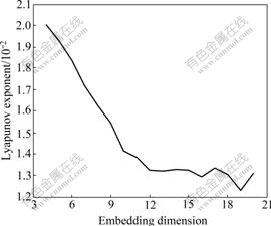
Fig.3 Lyapunov exponent (��) changing with embedding dimension (m)
6.3 Prediction process
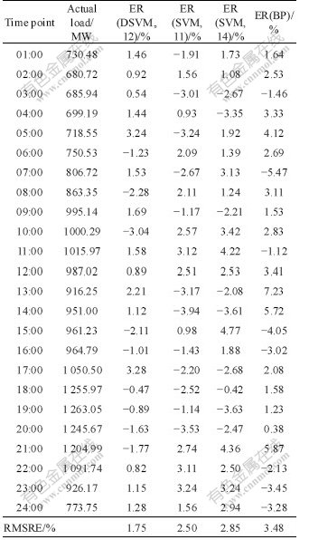
SVM is used to make prediction after the samples are normalized. Matlab7.1 is used to compute the results and radial basis function is chosen as the kernel function. The parameters are chosen as follows: m=12, C=79.31, ��=0.012, ��2=4.28. The other two comparing matrixes are established by choosing the parameters as follows: m=11, C=73.01, ��=0.017, ��2=2.13 and m=14, C=26.30, ��=0.006, ��2=1.60. The results of each matrix are shown in Table 3.
BP algorithm is used to make prediction with sigmoid function. The parameters are chosen as follows: the node number of input layer is 11 and the node number
of output layer is 1. The node number of interlayer is 8 according to the experience. The system error is 0.001 and the maximal interactive times is 5 000. The results are shown in Table 3.
Table 3 DSVM forecasting results and comparison
6.4 Predicted values and evaluating indicator
Relative error (ER) and root-mean-square relative error (RMSRE) are used as the final evaluating indicators:
![]() ��100% (9)
��100% (9)

The results are shown in Fig.4.
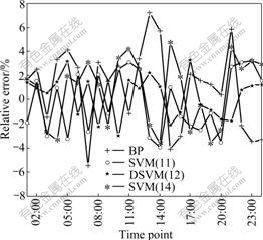
Fig.4 Error analysis with different models
To see whether the approach of choosing embedding dimension is reasonable or not, three cases are chosen as follows: 12-dimension based on data mining, less than 12-dimension that is 11-dimension and larger than 12-dimension that is 14-dimension. If the relative errors are measured by the standard that is 3%, the acceptable results in the condition of 12-dimension cover 87.50% while those of 11-dimension and 14-dimension cover 66.67% and 62.50%, respectively. If the results are measured by RMSRE, RMSRE of 12-dimension is less than that of the other two dimensions. It can be seen from the above analysis that the predicting effectiveness of 12-dimension is better than that of other dimensions when SVM is used to make prediction.
The comparison between SVM and BP is shown as follows: The RE of predicted results by SVM has small rangeability. The maximal RE is 3.28% and the value from the maximal RE to the minimal RE is 6.32%. On the contrary, the RE of predicted results by BP has large rangeability. The ratio of maximal RE to the minimal RE is 12.70%. If the results are measured by the standard that is less than or equal to 3%, the acceptable results of SVM will be 87.50%, while those of BP are 50%. If the results are measured by RMSRE, RMSRE of SVM will be less than that of BP. It can be seen from the above analysis that the predicting effectiveness of SVM is better than that of BP.
7 Conclusions
(1) The power load data show apparent chaotic character. Chaotic time series is established and chaotic parameters are computed, and then SVM based on data mining prediction model is established to make prediction. The real load data prediction shows that the model is effective in short-term power load forecasting.
(2) The embedding dimension is chosen through Lyapunov method. The predicted results with chosen dimension and other random dimensions are compared. Through comparison, it can be seen that the new model is scientific and rational. The results show that there is a suitable embedding dimension that can be used to predict the power load effectively. The predicted values computed by the model with a chosen dimension are highly accurate.
(3) It is necessary to preprocess the data that are seriously influenced by uncertain factors for short-term power load forecasting. The past loading data can be classified into different groups according to different characters and choosing finite sample points that have the same character to forecast with data mining technology. Then, SVM prediction model is established to make prediction. The real load data prediction based on Lyapunov exponents and data mining shows that the model is effective in short-term power load forecasting.
References
[1] CHRISTIANSE W R. Short term load forecasting using general exponential smoothing [J]. IEEE Trans Power Apparatus Syst, 1971, 90(2): 900-911.
[2] PARK J H, PARK Y M, LEE K Y. Composite modeling for adaptive short-term load forecasting [J]. IEEE Transactions on Power Systems, 1991, 6(2): 450-457.
[3] PAI Ping-feng, HONG Wei-chang. Support vector machines with simulated annealing algorithms in electricity load forecasting [J]. Energy Conversion and Management, 2005, 46: 2669-2688.
[4] NIU Dong-xiao, CAO Shu-hua, LU Jian-chang, ZHAO Lei. Technology and application of power load forecasting [M]. 2nd ed. Beijing: China Power Press, 2009. (in Chinese)
[5] MBAMALU G A N, EL-HAWARY M E. Load forecasting via suboptimal seasonal autoregressive models and iteratively reweighted least squares estimation [J]. IEEE Transactions on Power Systems, 1993, 8(1): 343-348.
[6] DOUGLAS A P, BREIPOHL A M, LEE F N, ADAPA R. Impacts of temperature forecast uncertainty on Bayesian load forecasting [J]. IEEE Transactions on Power Systems, 1998, 13(4): 1507-1513.
[7] SADOWNIK R, BARBOSA E P. Short-term forecasting of industrial electricity consumption in Brazil [J]. Journal of Forecasting, 1999, 18(3): 215-224.
[8] SU Cheng-jian. Study of nonlinear behavior on price and volatility of Chinese stock markets [J]. Mathematics in Practice and Theory, 2006, 36(2): 141-148.
[9] KATARZYNA B, ARKADIUSZ O. Application of bootstrap to detecting chaos in financial time series [J]. Physica A: Statistical Mechanics and its Applications, 2004, 344(2): 317-321.
[10] NU Jin-hu. Chaos time series analysis and its application [M]. Wuhan: Wuhan University Press, 2002. (in Chinese)
[11] CHEN Su-yan, WANG wei. Chaos forecasting for traffic flow based on Lyapunov exponent[J]. China Civil Engineering Journal, 2004, 37(9): 96-99. (in Chinese).
[12] DOUGLAS A P, BREIPOHL A M, LEE F N, ADAPA R. Risk due to load forecast uncertainty in short term power system planning [J]. IEEE Trans Pow Syst, 1998, 13(4): 1493-1499.
[13] VAPNIK V N. The nature of statistical learning theory [M]. New York: Springer, 1995.
[14] CORTES C, VAPNIK V. Support vector networks [J]. Mach Learn, 1995, 20(3): 273-297.
[15] HUANG W, NAKAMORI Y, WANG S Y. Forecasting stock market movement direction with support vector machine [J]. Computers and Operations Research, 2005, 32(10): 2513-2522.
[16] PAI Ping-feng, HONG Wei-chang. Software reliability forecasting by support vector machines with simulated annealing algorithms [J]. J Syst Software, 2006, 79(6): 747-755.
[17] CATALAO J P S, MARIANO S J P S, MENDES V M F, FERREIRA L A F M. Short-term electricity prices forecasting in a competitive market: A neural network approach [J]. Electric Power Systems Research, 2007, 77(10): 1297-1304.
[18] WOLF A, SWIFT J B, SWINNEY H L. Determining Lyapunov exponents from a time series [J]. Physics D, 1985, 116: 285-317.
[19] LIANG Zhi-shan, WANG Li-ming, FU Da-peng, Short-term power load forecasting based on Lyapunov exponents [J]. Proceeding of the CSEE, 1998, 118: 368-472.
[20] NIU Dong-xiao, WANG Yong-li, WU De-sheng. Power load forecasting using support vector machine and ant colony optimization [J]. Expert Systems with Applications, 2010, 37(3): 2531-2539.
[21] NIU Dong-xiao, WANG Yong-li, DUAN Chun-ming, XING Mian. A new short-term power load forecasting model based on chaotic time series and SVM [J]. Journal of Universal Computer Science, 2009, 15(13): 2726-2745.
Foundation item: Project(70671039) supported by the National Natural Science Foundation of China
Received date: 2009-06-08; Accepted date: 2009-10-20
Corresponding author: NIU Dong-xiao, PhD, Professor; Tel: +86-10-80796652; E-mail: niudx@126.com
(Edited by CHEN Wei-ping)
Abstract: According to the chaotic and non-linear characters of power load data, the time series matrix is established with the theory of phase-space reconstruction, and then Lyapunov exponents with chaotic time series are computed to determine the time delay and the embedding dimension. Due to different features of the data, data mining algorithm is conducted to classify the data into different groups. Redundant information is eliminated by the advantage of data mining technology, and the historical loads that have highly similar features with the forecasting day are searched by the system. As a result, the training data can be decreased and the computing speed can also be improved when constructing support vector machine (SVM) model. Then, SVM algorithm is used to predict power load with parameters that get in pretreatment. In order to prove the effectiveness of the new model, the calculation with data mining SVM algorithm is compared with that of single SVM and back propagation network. It can be seen that the new DSVM algorithm effectively improves the forecast accuracy by 0.75%, 1.10% and 1.73% compared with SVM for two random dimensions of 11-dimension, 14-dimension and BP network, respectively. This indicates that the DSVM gains perfect improvement effect in the short-term power load forecasting.
