
J. Cent. South Univ. (2016) 23: 2926-2934
DOI: 10.1007/s11771-016-3356-x

Comparison of dynamic Bayesian network approaches for online diagnosis of aircraft system
YU Jin-song(�ھ���)1, 2, FENG Wei(����)1, TANG Di-yin(��ݶ��)1, LIU Hao(����)1, 3
1. School of Automation Science and Electrical Engineering, Beihang University, Beijing 100191, China;
2. Collaborative Innovation Center of Advanced Aero-Engine, Beihang University, Beijing 100191, China;
3. Unit 93, Army 95809 of PLA, Cangzhou 061736, China
 Central South University Press and Springer-Verlag Berlin Heidelberg 2016
Abstract:
The online diagnosis for aircraft system has always been a difficult problem. This is due to time evolution of system change, uncertainty of sensor measurements, and real-time requirement of diagnostic inference. To address this problem, two dynamic Bayesian network (DBN) approaches are proposed. One approach prunes the DBN of system, and then uses particle filter (PF) for this pruned DBN (PDBN) to perform online diagnosis. The problem is that estimates from a PF tend to have high variance for small sample sets. Using large sample sets is computationally expensive. The other approach compiles the PDBN into a dynamic arithmetic circuit (DAC) using an offline procedure that is applied only once, and then uses this circuit to provide online diagnosis recursively. This approach leads to the most computational consumption in the offline procedure. The experimental results show that the DAC, compared with the PF for PDBN, not only provides more reliable online diagnosis, but also offers much faster inference.
Key words:
online diagnosis; dynamic Bayesian network; particle filter; dynamic arithmetic circuit��
1 Introduction
Safety is always the fundamental issue of flights all over the world. Industry and governments have endeavored to reduce the number of accidents for commercial aircraft, however, investigation data [1] from International Civil Aviation Organization (ICAO) show increasing rates of accident from 90 in 2013 to 98 in 2014 during 2012-2014 period of time, which caused 372, 173 and 906 fatalities, respectively. According to the accident investigation, the aircraft system failures are recognized as one of the most important causes. Hence, it is necessary to develop an effective online diagnosis to reduce the probability of its fault occurrence and consequent fatalities.
In general, the online diagnosis for aircraft system has always been a difficult problem. This is due to time evolution of system change, uncertainty of sensor measurements, and real-time requirement of diagnostic inference. These factors result in the corresponding online diagnosis providing fast, predictable, and reliable inference, so that the faults in the system must be detected before they lead to catastrophic failures.
Over the years, various researches have contributed enormously to solving this problem. Probabilistic Bayesian networks, e.g., Bayesian networks (BNs) [2], hidden Markov models (HMMs) [3], Kalman filter models (KFMs) [4], dynamic Bayesian network (DBN) [5], offer a mathematically sound basis for making inferences under the presence of uncertainty, whose conditional probability tables (CPTs) provide a natural way to represent uncertain events, and the semantics of the updated probabilities are well-defined. Among them, BNs occupy a prominent position in artificial intelligence (AI), but BNs are static models, hence the dynamic system cannot be easily represented using BNs [6]. HMMs have been used in a wide range of applications and worked very well in practice [7-9], but these models require an exponential number of parameters to specify their transition and observation models, and in addition, the inference by HMMs takes exponential time [10]. KFMs offer an recursive means to estimate the state of a process, even when the precise nature of the modeled system is unknown [11]. But KFMs assume that the system is jointly Gaussian. This means that the belief state must be unimodal, which is inappropriate for many problems, especially those involving qualitative (discrete) variables [10]. DBN, an extension of the BN, can overcome these limitations above by representing the evolution of the cascading events in a more physical way [12]. Many Bayesian inference algorithms can be applied for DBN to generate consistent diagnostic result in a recursive manner. But the exact inference, suffering from expensive computation problem, is also intractable. It is worth noting that BNs inference problem is also inherently computationally hard [13-14]. One effective solution for this problem is the differential approach [15-16], where a BN is compiled into a (static) arithmetic circuit (AC) using an offline phase, and then this circuit can be used for online real-time diagnosis. However, the AC encounters the same limitation as BNs: none of them provides direct mechanism for representing dynamic systems.
In this work, two novel approaches are proposed to address this problem as follows:
1) PF on pruned DBN (PDBN): According to the independence rule of DBN, the DBN can be simplified by pruning some nodes in its first time slice. To apply PF to the resulting PDBN, the likelihood weighting (LW) algorithm [17] is used to generate particles and their weights, and then optimal estimates can be obtained. The problem is that estimates from a PF tend to have high variance for small sample sets. Using large sample sets is computationally expensive [18].
2) Compilation of PDBN: The differential approach can be extended to PDBN, i.e., the PDBN is compiled into dynamic arithmetic circuit (DAC) using an offline procedure that is applied only once, and then this circuit can be recursively used for online diagnosis at each time step. The separation of inference process into offline and online procedures leads to the most computational consumption in the offline procedure.
The effectiveness of both approaches above is verified through experiment on a real-world aircraft fuel delivery system (AFDS). The results show that the DAC not only provides online diagnosis recursively, but also satisfies the real-time constrains.
2 Development of pruned DBN
For an aircraft system, its DBN can be automatically generated using an object-oriented approach [19]. Figure 1 depicts a DBN that represents the voltage sensor and switch components, which is the fragment of the resulting DBN for a real-world AFDS.
In this model, the nodes Hs are defined as persistent nodes [10] (i.e., the nodes are used to accumulate the temporal causal influence). Note DBN can contain both discrete and continuous random variables; but our work considers discrete variables only, hence, all sensor measurements, which are usually time-series signals under uncertainty, must undergo a preprocessing phase (e.g., sampling and discretization), where certain features are extracted. The DBN encodes two independent rules:
1) The future is independent of the past given the present (i.e., first-order Markov assumption).
2) Each node X in the model is independent of its non-descendants given its parents node, Pa(X).
Consider again the DBN in Fig. 1. In this model, the health nodes Hs are persistent nodes. Hence, before the model evolves new time t+1, the influence accumulated before time t must be absorbed into health nodes Hs in the first slice. This is accomplished by revising their CPTs with the posterior probability distribution updated in the most recent time. Meantime, the health nodes Hs are root nodes. Hence, the revised CPTs are not affected by other nodes within the same slice. At this time, the DBN represents a snapshot of system behavior in two consecutive time slices, t and t+1.
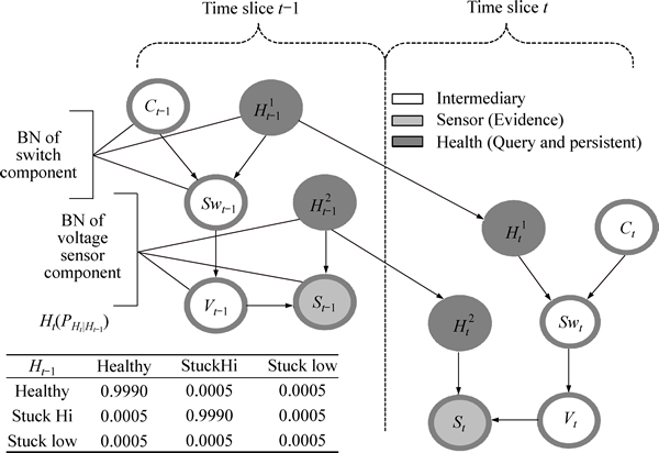
Fig. 1 DBN of voltage sensor and switch components
Definition 1 (PDBN): Let D be a DBN composed of two consecutive time slices (i.e., t-1, t). The PDBN D' is obtained from D by pruning any node (with its CPT) in time slice t-1 as long as it does not belong to Hst-1 nodes. With the time evolution, the CPT of each H t-1 must be revised by the posterior probability distribution updated in the most recent time.
Theorem 1: Let D be a DBN, D' is its PDBN, and let (Ht, st) be a query, then P(Ht | St, Ht-1)= P'(Ht |St, Ht-1), where P and P' are the posterior probability distribution updated by networks D and D', respectively.
Figure 2 depicts the corresponding PDBN for DBN in Fig. 1. The PDBN seems to be a simple version of DBN, leading to less computation consumption in online diagnosis of both DBN approaches.
3 PF on PDBN
Consider again the PDBN in Fig. 2 and assume that our goal is to estimate the posterior probability distribution P(h|s) for each time t. The key insight behind PF is to use likelihood-weighting algorithm for the network fragments (see Fig. 3) that allow us to efficiently perform following processes:
Step 1: The initial probability distribution P(H1) is represented by a DBN fragment depicted in Fig. 3(a). Hence, an initial set of particles for time t=1 can be sampled by applying Monte-Carlo sampling approach [20] to this network.
Step 2: The probability distribution  can be represented by a DBN fragment as shown in Fig. 3(b). The particles for time t>1 can be generated from the particles for time t-1 by applying Monte-Carlo sampling approach to this network.
Step 3: The probability distribution  can be represented by a DBN fragment shown in Fig. 3(c). Based on this fragment, the weight of each particle can be calculated efficiently. Subsequently, given the sensor measurements s for time t, calculating the posterior probability distribution
  becomes straightforward, which is given by

 (1)
(1)
where m denotes the number of sensor components, and n denotes the sample size.
Step 4: The CPTs of Hs in the first slice of PDBN are revised using the calculated posterior probabilities distribution , and then new particles can be resampled from these nodes. At this time, the PDBN represents a snapshot of system behavior in two consecutive time slice, t and t+1.
The detail information is summarized in Fig. 4. With sufficient particles, this approach can provide accurate online diagnosis for each time t>1, but may bring expensive computation problem.

Fig. 2 PDBN of voltage sensor and switch
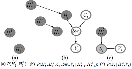
Fig. 3 Fragments of the PDBN in Fig. 2:
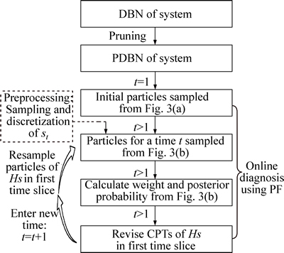
Fig. 4 Flow chart of online diagnosis using PF
4 Compilation of PDBN
4.1 Network polynomial of PDBN
For each PDBN, its probability distribution can be represented as a network polynomial f, which is defined as follows.
Definition 2 (PDBN network polynomial): Let D' be a PDBN over variables V, and let Hst-1 be the set of nodes in time slice t-1; Y be the set of nodes in time slice t; U be the parents of Y; lV be the set of indicators for V; dH be the temporal parameters for Hst-1; qY|U be the set of network parameters for Y. The network polynomial of D'is composed of lV, dH, and qY|U as
 (2)
(2)
where for each instantiation v, the inner product ranges over lV, dH, and qY|U variables that are consistent with v (i.e., ��~�� denotes the compatibility relationship among instantiations); the outer sum ranges over all instantiations v of the network nodes.
For example, let us consider a simple PDBN in Fig. 5, which is the fragment of PDBN in Fig. 2. Note that the network polynomial of this network has thirty- six terms, some of which are presented below:

Fig. 5 Fragment of PDBN in Fig. 2


 (3)
(3)
where variables h,  and
and  respectively denote each state of H.
The network polynomial in Eq. (3) can be viewed as a particular representation for the joint probability distribution induced by the PDBN in Fig. 5, where each term is in one-to-one correspondence with the rows of the network��s joint distribution. This polynomial can be used to represent the probability of any sensor measurement s by carefully setting certain indictors to 0, instead of 1, depending on whether they agree with s.
For example, if the sensor measurement is s at time t, then the corresponding indictors can be assigned as
 (4)
(4)
Finally, the value of Eq. (3) under these settings is equivalent to erase terms that contain  This results in the total number of terms being sixteen, some of which are shown as


 (5)
(5)
The network polynomial has an exponential size as it includes a term for each instantiation over the entire network variables. Therefore, any direct representation of the network polynomial for complex PDBN is infeasible. An efficient and comprehensive approach is to represent this network polynomial using DAC.
4.2 DAC development (offline phase)
4.2.1 DAC definition
To address the representation problem of network polynomial for PDBN, a well-designed DAC is proposed in this sub-section. Its inference takes time linear in circuit size, where size is defined as the number of edges in circuit.
Definition 3 (DAC): Let D' be a PDBN over variables V, and let Hst-1 be the set of nodes in time slice t-1; Y be all variables in time slice t; lV be the set of all indicators for V; dH be the temporal parameters for Hst-1; qY|U be the set of network parameters for Y. The DAC for D' is defined as a rooted DAG, where leaf nodes are labeled with constants or variables in ��=lV��qY|U��dH,and internal nodes are labeled with multiplication and addition operations.
Figure 6 depicts the DAC of the network polynomial in Eq. (3) (i.e., for PDBN in Fig. 5). Next, how to obtain this DAC will be described.
4.2.2 DAC construction
The join tree algorithm seems to be a variation of variable elimination (VE) algorithm, which improves in the complexity of VE used for Bayesian inference. Therefore, the join tree algorithm is chosen to generate DAC in this work.
Step 1: Build Join tree
A join tree for a DAG G of network N is a labeled tree (T, C, S), where T is a tree, each node in T is labeled with cluster Ci , and each edge is labeled with separator Sij. The join tree must satisfy the following properties:
1) Each cluster Ci is a set of nodes from G.
2) Each family XU must exist in some cluster.
3) If a variable X appears in two clusters, all clusters on the path between both clusters must contain X. This is known as join-tree property.
4) The separator of edge i-j is defined as Ci��Cj.
The construction of join tree T from DAG G involves a number of sub-steps, and can be summarized as
1) Build a moral graph of G.
2) Add edges to the moral graph for forming a triangulated graph based on elimination order.

Fig. 6 DAC for simple PDBN in Fig. 5
3) From the triangulated graph, identify subsets of nodes to form clusters.
4) Construct a join tree: connect the clusters to form an undirected tree satisfying the join-tree property, inserting the corresponding separator.
Sub-steps 2 and 4 are nondeterministic (e.g., there are different elimination orders). Hence, different join trees can be built from the same DAG. Figure 7 depicts the moral graph and a join tree for PDBN in Fig. 5, where the elimination order is {S, V, Ht, Ht-1}. Note that the triangulated graph is the same as moral graph given this order.

Fig. 7 Moral graph and join tree for PDBN in Fig. 5
Step 2: Build DAC using join tree
Before a join tree is used to build the DAC, each CPT (i.e., ��X|U) must be assigned to a cluster that contains the family XU. Meantime, the indicator lX for any variable X must be assigned to a cluster that includes X. Furthermore, a cluster in the join tree must be chosen as the root, allowing us to define parents/children relationships between neighbor clusters and separators. Hence, the join tree in Fig. 7 is converted into the equivalent one in Fig. 8 that depicts the root cluster, in addition to the assignment of ��X|U and lX to clusters.
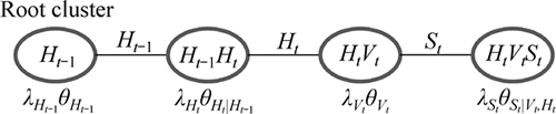
Fig. 8 Join tree for develop DAC
In fact, the DAC embedded in this join tree is defined as below, which contains:
1) One output addition node 
2) A multiplication node for each instantiation of a cluster Ci, represented as �� ��.
��.
3) An addition node for each instantiation of a separator Sij, represented as ��+��.
4) An input node lx for each instantiation x of variable X.
5) An input node dh for each instantiation h of nodes in time slice t-1.
6) An input node ��y|u for each instantiation yu of family YU, where Y is a variable in time slice t.
Figure 6 depicts the resulting DAC, whose join tree is shown in Fig. 8. Note that the temporal nodes dH are highlighted in this circuit with dark gray filled circle.
4.3 Online diagnosis using DAC
Once the DAC is constructed, the posterior probability distribution at each time step can be recursively calculated by proceeding variables setting, bottom-up evaluation, top-down differentiation, posterior updating, and probability revision.
Step 1: Variables setting
The DAC has three types of leaf nodes: temporal parameters dH, network parameters qY|U, and indicators lV. dH are set according to the initial prior probability distribution only at time t=1; qY|U are set according to the network CPTs; and lV are set according to the given sensor measurements at current time t��1.
Step 2: Bottom-up evaluation
Once the leaf nodes are set, the algebraic value of each node (excludes the leaf nodes) in this circuit can be evaluated using a bottom-up pass, which proceeds from its children to itself. If let {Y1, Y2, ��, Yn} be the children of an arbitrary node X, the algebraic value of node X at sensor measurements st, denoted by Vr(X), is defined as
 (6)
(6)
Note the value of root node, Vr(R), is guaranteed to be the probability of given sensor measurements st.
Step 3: Top-down differentiation
The differentiation process calculates the partial derivatives of the circuit root with respect to each circuit node X, which proceeds top-down from the node X to its children. Let Dr(X) denote the partial derivative of node X. If X is a leaf node, its partial derivative represents the change in the circuit root for each unit change in X. In particular, for each indicator lx, there is
 (7)
(7)
Now, let the partial derivative of root node be initialized to 1, and that of others be initialized to 0. If X is not the root node, and its parent P is a multiplication node, then


 (8)
(8)
Similarly, its parent P is an addition node,

 (9)
(9)
Furthermore, if let m stand for the number of addition parents, and let n stand for the number of multiplication parents, then
 (10)
(10)
In this manner, the partial derivatives of the circuit root with respect to any leaf node can be calculated.
Step 4: Posterior updating
Once the partial derivatives for indictors of health nodes are obtained, updating the corresponding posterior probability distribution at sensor measurements st becomes straightforward, which is represented next.


 (11)
(11)
Step 5: Probability revision
Before the circuit enters a new time, the value of temporal nodes (i.e., dh) must be revised immediately using the posterior probability distribution updated by Eq. (11). In this way, the historical influence accumulated over time is always integrated into this DAC.
Overall, the compilation of PDBN approach, specifically designed for online diagnosis of aircraft system, is summarized in Fig. 9.
5 Results and discussion
To explicitly verify both DBN approaches discussed above, all attentions will be focused on a real-world AFDS in Fig. 10. As depicted, this system comprises two independent auxiliary tanks (1-2) with dedicated pumps (1-2) feeding a main tank. The electric power circuitry to the pumps along with controller and an extensive set of measurement devices (sensors and monitors) make up the rest of the system.
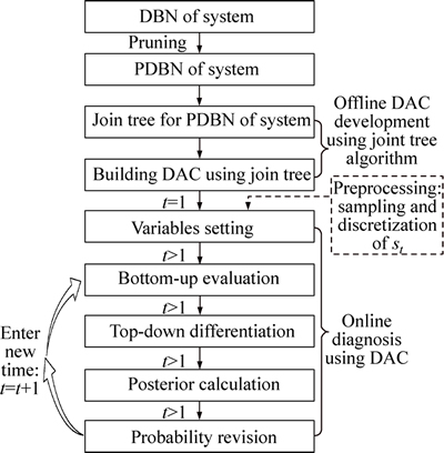
Fig. 9 Flow chart of compilation of DBN
Table 1 presents the health parameters of possible faulty components. Note all of them are discretized into symbolic states (e.g., health, leak, block, etc.) with normalized probability values to present current states of components.
The DBN, PDBN and DAC of this AFDS contain over 70, 50 and 1300 nodes, respectively. In order to achieve correct posterior estimation, the experiment must satisfy the following requirements:
1) In the initial state, all components stay in healthy state.
2) The fuel level of the main tank is lower than the preset alarm threshold, i.e., the level sensor 1 is clamped to low state (i.e., SL1=2).
3) The fuel level of each auxiliary tank is higher than the preset alarm threshold, i.e., the level sensor 2 and sensor 3 are clamped to high state (i.e., SL2=1, SL3=1).
4) Switch 1 is supposed to be closed, and switch 2 is supposed to be opened (i.e., SP1=1, SP2=2).
In our experiment, the fault is injected in pump 1 component at time: t=11-13; t=31-34. The corresponding sensor measurements are: st={SL1=2, SL2=1, SL3=1, SV1=1, SV2=1, SV3=1, SV4=2, SP1=1, SP2=2, M1=2, M2=2}.
Figure 11 depicts the diagnostic result using DAC, where a negative deviation, represented as the cyan right- pointing triangle curve, is first captured at time t=11. When the fault disappears at time t=14, the DAC can quickly capture this change and precisely track the real states of the system. If the fault appears only once, this negative deviation may be recognized as a false alarm; however, the fault appears again at time t=31. The DAC can also immediately detect and track the fault again. Hence, the result obtained is consistent with our fault scenario.

Fig. 10 Structure of AFDS
Table 1 Health parameters of AFDS


Fig. 11 Online diagnosis using DAC
The PF can also be used to detect and isolate this fault online, whose diagnostic results of DBN and PDBN are all the same. Figure 12 depicts the corresponding diagnostic results for PDBN, where two curves agree with the fault scenario. The PF with 1000 particles can provide more reliable online diagnosis than PF with 500 particles. Note that the curves of other components that operate normally are omitted for clearer presentation.
Moreover, the diagnostic curve in Fig. 11 is much more accurate than that in Fig. 12. This indicates that the DAC can offer more reliable online diagnosis.

Fig. 12 Online diagnosis using PF on DBN/PDBN
Table 2 Online diagnosis results with order of measurements of SL1, SL2, SL3, SV1, SV2, SV3, SV4, SP1, SP2, M1, M2
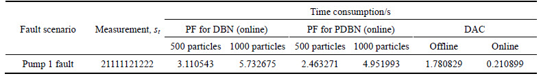
Table 2 summarizes the computational consumption of both DBN approaches. For example, the average computation of each time step used by PF with 1000 applied on DBN and PDBN is 5.732675 s and 4.951993 s, respectively, which is much more than 0.210899 s used by DAC. These data lead to a conclusion that the DAC can offer fast online inference.
6 Conclusions
1) Based on the independence rule of DBN, the DBN can be simplified by pruning some nodes in the first time slice. This process leads to less computational consumption in online diagnosis of both DBN approaches.
2) With sufficient particles, the particle filter (PF) for pruned DBN (PDBN) can obtain a Bayesian optimal estimate. However, estimates tend to have a high variance for small sample sets; using large sample sets may otherwise suffer from expensive computation problem.
3) The compilation of PDBN approach provides more effective and efficient online diagnosis. In this approach, the PDBN is compiled into a dynamic arithmetic circuit (DAC) using an offline phase that is applied only once, and then this circuit can offer reliable and fast online diagnosis recursively. The separation of the inference process into offline and online phases results in the most computational consumption in the offline phase, thereby meeting the real-time requirements.
References
[1] ICAO. Annual Report 2014[EB/OL]. http://www.icao.int/annual- report-2014/Pages/the world of air transport in 2014.aspx.
[2] ZHANG Q Q, XU Y P, TIAN Y, ZHANG X J. Risk-based water quality decision-making under small data using Bayesian network [J]. Journal of Central South University, 2012, 19: 3215-3224.
[3] CHAN A D, ENGLEHART K B. Continuous myoelectric control for powered prostheses using hidden Markov models [J]. Biomedical Engineering, IEEE Transactions on, 2005, 52(1): 121-124.
[4] YUAN L, SHEN J Q, XIAO F, WANG H L. A novel reaching law approach of quasi-sliding-mode control for uncertain discrete-time systems [J]. Journal of Central South University, 2012, 19: 2514-2519.
[5] PALUSZEWSKI M, HAMELRYCK T. Mocapy++-A toolkit for inference and learning in dynamic Bayesian networks [J]. BMC Bioinformatics, 2010, 11(1): 126.
[6] ROYCHOUDHURY I. Distributed diagnosis of continuous systems: Global diagnosis through local analysis [D]. Nashville Tennessee: Vanderbilt University, 2009.
[7] YUAN L C. Improved hidden Markov model for speech recognition and POS tagging [J]. Journal of Central South University, 2012, 19: 511-516.
[8] WANG L, CAI Z X. Place recognition based on saliency for topological localization [J]. Journal of Central South University of Technology, 2006, 13(5): 536-541.
[9] ZHU S R. Authentication based on feature of hand-written signature [J]. Journal of Central South University of Technology, 2007, 14: 563-567.
[10] MURPHY K P. Dynamic bayesian networks: representation, inference and learning [D]. University of California, 2002.
[11] WELCH G, BISHOP G. An introduction to the Kalman filter [C]// Proceeding of Siggraph'95. New York: USA: New York: ACM press, 1995: 1-16.
[12] MURPHY K P, PASKIN M A. Linear-time inference in hierarchical HMMs [J]. Advances in Neural Information Processing Systems, 2002, 2(1): 833-840.
[13] GUO H, HSU W. A survey of algorithms for real-time Bayesian network inference [C]// AAAI Joint Workshop on Real-Time Decision Support and Diagnosis Systems. Edmonton, Canada: Alberta: AAAI Press, 2002: 1-12.
[14] TEYSSIER M, KOLLER D. Ordering-based search: A simple and effective algorithm for learning Bayesian networks [C]// Proceedings of the 21st Conference in Uncertainty in Artificial Intelligence. Edinburgh, Sctland, 2005: 584-590.
[15] MENGSHOEL O J, DARWICHE A, CASCIO K, CHAVIRA M, POLL S, UCKUN S. Diagnosing faults in electrical power systems of spacecraft and aircraft [J]. Association for the Advancement of Artificial Intelligence, 2008, 3(1): 1699-1705.
[16] DARWICHE A. A differential approach to inference in Bayesian networks [J]. Journal of the ACM (JACM), 2003, 50(3): 280-305.
[17] BIDYUK B, DECHTER R. Cutset Sampling with Likelihood Weighting [C]// Proceedings of the 22nd Conference in Uncertainty in Artificial Intelligence. Cambridge, MA, USA, 2006: 489-500.
[18] VERMA V, GORDON G, SIMMONS R, THRUN S. Real-time fault diagnosis [robot fault diagnosis] [J]. Robotics & Automation Magazine, IEEE, 2004, 11(2): 56-66.
[19] FENG W, YU J S, LI J, LIU H. Bayesian health modeling for aerial dynamic system using object-oriented approach [J]. Proceedings of 2013 IEEE 11th International Conference on Electronic Measurement & Instruments, 2013, 2: 837-842.
[20] RUBINSTEIN R Y, KROESE D P. Simulation and the Monte Carlo method [M]. Wiley, 2011: 5-101.
(Edited by YANG Bing)
Foundation item: Projects(2010ZD11007, 20100751010) supported by Aeronautical Science Foundation of China
Received date: 2015-07-15; Accepted date: 2015-12-24
Corresponding author: YU Jin-song, Associate Professor, PhD; Tel: +86-10-82338693; E-mail: yujs@buaa.edu.cn
Abstract: The online diagnosis for aircraft system has always been a difficult problem. This is due to time evolution of system change, uncertainty of sensor measurements, and real-time requirement of diagnostic inference. To address this problem, two dynamic Bayesian network (DBN) approaches are proposed. One approach prunes the DBN of system, and then uses particle filter (PF) for this pruned DBN (PDBN) to perform online diagnosis. The problem is that estimates from a PF tend to have high variance for small sample sets. Using large sample sets is computationally expensive. The other approach compiles the PDBN into a dynamic arithmetic circuit (DAC) using an offline procedure that is applied only once, and then uses this circuit to provide online diagnosis recursively. This approach leads to the most computational consumption in the offline procedure. The experimental results show that the DAC, compared with the PF for PDBN, not only provides more reliable online diagnosis, but also offers much faster inference.
