J. Cent. South Univ. Technol. (2011) 18: 1619-1625

DOI: 10.1007/s11771-011-0881-5

Strain field investigation of limestone specimen under uniaxial compression loads using particle image velocimetry

XU Jin-ming(徐金明)¹, CHENG Chang-hong(程昌宏)¹, LU Hai-ping(陆海平)²

1. Department of Civil Engineering, Shanghai University, Shanghai 200072, China;

2. Hunan Zhongda Design Institute Company Limited,

Central South University, Changsha 410075, China

? Central South University Press and Springer-Verlag Berlin Heidelberg 2011

Key words:

rock materials; limestone; video image; strain field; uniaxial compression; particle image velocimetry；

1 Introduction

The mechanical properties, such as the displacements and strains, of rock materials play an important role in practice. In conventional methods, these properties were investigated using laboratory tests, and most often, using the uniaxial compression tests in laboratory. With the development of the computer techniques in the last 30 years, these properties have been explored using the digital image analysis and related techniques.

The digital image processing method is a tool that permits a fast and accurate acquisition of information of mechanical properties. There are many approaches in the evaluation of applicable algorithms that extract the displacement and strain fields from photographic static images or video images. DEB et al [1] analyzed the discontinuity geometry of rock mass exposures, and recommended a digital face mapping method to characterize rock masses. XU et al [2] presented the digital image analysis of fluid inclusions in rocks, and investigated the characteristics of fluid inclusion lines using edge-detection techniques and mathematical morphological analyses. YIN et al [3] utilized the sequential damage images of geomaterials offered by computerized tomography (CT) technology to obtain the locations of cracks. Taking the light intensity pattern from the scanning electron microscope (SEM), ZHAO  et al [4] performed a correlation computation to evaluate the deformation field of a fine grain sandstone surface involving the micro-cracks. Using the colorful video images and experimental data from the laboratory uniaxial compression test of a limestone, XU et al [5] obtained the displacement field using a digital image correlation (DIC) technique. WANG et al [6] measured the strain field of a deforming sheet using the digital image analysis and argued the key aspects of the grid recognition. CHEN et al [7] obtained the geometrical parameters and the strains of a deformed square grids using digital image analysis. SHAO et al [8] provided a means with digital image processing technique for exploring the local deformation process of soil specimen in triaxial test. WANG et al [9] utilized the moire interferometry method to investigate the strain concentration factor of a carbon fiber composite plate with a central hole.

The particle image velocimetry (PIV) technique has also been applied in exploring the deformation properties of geomaterials. ADAM et al [10] monitored the displacement field in scaled tectonic model experiments using high-resolution optical image correlation techniques and obtained much valuable information. CASTELLUCCIO et al [11] employed an open source code, MATPIV, to examine the displacements and strains of SEM images by measuring the position in a regular grid. WOLF et al [12] utilized the X-ray technique and the PIV-based method to investigate the formation and changes of the shear band patterns in a granular structure. NIEDOSTATKIEWICZ et al [13] investigated the evolution of shear zones in cohesionless sand for the earth pressure problem of a retaining wall using PIV, and the effect of initial sand density on distribution of volumetric and deviatoric strain. WHITE et al [14] developed a deformation measurement system based on PIV and close-range photogrammetry to measure the movement of a fine mesh of soil patches. BHANDARI and INOUEN [15] examined the developing and transiting mechanism of strain localization deformation inside soft rock specimens using plane strain tests and finite element simulations. ZHANG et al [16] presented a microscopic measuring method for observing the movement of soil particles at sub-pixel accuracy from the image series during a soil-structure interface test.

Although the PIV-based method has been used in many fields, the applications in the field of geological engineering were limited. In the current study, the PIV method was used to investigate the full-field displacements and strains on the specimen surface under external loads from the video images captured in the uniaxial compression tests. Codes were developed using the MATLAB software in conducting the digital image processing.

2 Computation of displacement field

2.1 Laboratory tests and image acquisition

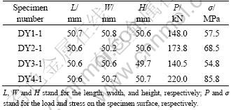
The limestone used in the current study was obtained from the Baiheling slope, located in Huzhou City, Zhejiang Province, China. The rock was sliced and polished into the cubic specimens with the size of around 50 mm × 50 mm × 50 mm. The uniaxial compression tests for the specimens were employed using the YE-2000 type hydraulic machine, produced by the Zhejiang Jingyuan Machinery Company Limited, China. The external stress data on the plate were acquired using the SmartTest Computer-controlled System. Table 1 presents the results of uniaxial compression tests for the limestone specimen.

Table 1 Results of uniaxial compression tests for limestone specimen

In this study, digital images from a digital camera were acquired by leveling it normal to the rock specimen surface. The distances from the camera to the specimens were about 5.0 m. The deformation in the experiments was recorded by the sequential digital images. All photographs were taken using a Sony Cybershot DSC-W5 digital camera with a sensor resolution of 5.0 mega pixels. In this study, the above-mentioned camera was used and placed normal to the rock exposure to be mapped in order to eliminate the perspective errors and lens distortion. Table 2 presents the summary of video images for the limestone specimens.

Table 2 Summary of video images for limestone specimen

2.2 Computation of displacement field

2.2.1 Theory background of PIV technique

To implement the later computations, the original video images were first converted into ones in a readable format. The frame images were then extracted from the readable video images.

To determine the displacement distributions on the surface of the limestone specimens, digital pictures of the specimen were taken and evaluated with an image analysis technique, called Particle Image Velocimetry (PIV). PIV is an optical technique for measuring the displacement fields in fluid mechanics, based on the pattern matching from the fluid videos with suspended particles. This technique has been used as a general tool to measure the displacements and, in essence, does not depend whether images correspond to fluids or solids. Hence, it can be a useful tool to analyze the inhomogeneous deformation of solids. In comparison with well-known examples of image processing, such as laser speckle technique, computed tomography and stereo-photo-grammetry, the PIV-method can be used to calculate the displacement field of the side of the specimen. Instead of measuring at only one point in the solids, PIV has the ability to capture the displacement distributions for a full-field simultaneously with high resolution.

In PIV, the displacement in a body is measured in the plane of the image and inferred from two consecutive images, separated by a time distance. After dividing both images into smaller regions or sub-windows, each sub-window in the first image was compared with a sub-window in the second image. For every possible overlap of the sub-windows, the sum of the squared difference between them was calculated. This is a criterion to define the position for which sub-window was the “least unlike”. The local displacement vectors are calculated for small sub-windows of the images by means of cross-correlation. The digital cross-correlation yields an average of the local displacement vector over the size of the sub-window. The highest value in the correlation plane can then be used as a direct estimate of the image displacement. The full-field displacement field consists of the vectors of all sub-windows.

2.2.2 Computing displacements using MATPIV

The open libraries from the MATPIV project, an application of the PIV theory using MATLAB scripts, were adapted for measuring the displacements and strains on the limestone specimen images. In this study, the tensile displacements were defined as positive ones, while the compressive displacements were defined as negative ones.

In MATPIV, the video images were interrogated in multi passes using different sizes of sub-windows with different overlaps. The calculation starts with relatively large sub-windows and refines the calculation using smaller sub-windows. In using MATPIV, each frame was taken using the window shifting technique. We started off with 64 × 64 images, ended with 16 × 16 images after 6 iterations, and utilized 75% overlap of the sub- windows.

2.2.3 Filtering displacements

After the above calculations are completed, it is usually necessary to filter the displacement data in order to remove the spurious vectors, which occurs primarily due to low image quality in some parts of the images. This was done in modified MATPIV using four filters: signal-to-noise ratio filter, peak height filter, global filter, and local filter.

In the signal-to-noise ratio (SNR) filter, all of the “invalid” displacement vectors (with a SNR lower than a threshold) were replaced with NAN, or “Not A Number”. In the peak height filter, unreliable vectors were replaced by interpolating from the valid neighbors if the ratio of the largest to the second largest peak exceeded a threshold. In the global filter, vectors that were significantly larger or smaller than a majority of the vectors would be removed. In the local filter, two local filters were commonly used: a median filter and a mean filter. They filtered displacements based on the squared difference between individual displacement vectors and the median or the mean of their surrounding neighbors.

As for the local filter, the median filter was used in the current study. In the median filter, if the difference between the median and the existing magnitude of vectors was greater than the specified threshold, the existing displacement would be considered as an outlier and replaced by NAN. In this case, the displacement U_{i, j} does not belong to the interval of [U₁, U₂], where

                                                      (1)

where M and S are the median and standard variations of the displacements at the pixel locations between (i-1, j-1) and (i+1, j+1); T is a threshold specified to be 3 in this study.

If NAN was encountered, the displacement at the point was computed using the cubic interpolation. All of the spurious vectors were sorted based on the number of their neighbors and started by interpolating the vector that had as few neighboring outliers as possible, looping until no NAN remained.

The displacement fields were filtered to remove the spurious vectors. The missing vector values were replaced using a cubic interpolation. Figure 1 presents the displacement fields before and after filtering. It can be seen that the displacement field was smoother after filtering than that before filtering.

The displacement was the integral multiple of pixel values when using the cross correlation technique. Because the position in the query window after deformation had occurred was not definitely an integer, the sub-pixel measurement technique was furthermore used in this study. This technique cannot improve the resolution of the studied image but can make the result displacements better coincided with actual ones. In the current study, the maximum correlation coefficient was computed in the sub-pixel level. The correlation coefficients were distributed in a Gaussian form around a point having the maximum value, and the Gaussian fit was used to estimate the displacements in the adjacent area of the point. The point with the maximum value was selected as the objective sub-pixel position. By using the Gaussian fit technique and the correlation coefficients at the maximum point and its surrounding four points, the displacement at the sub-pixel position was determined using the maximum value of the correlation coefficients computed by

    (2)

where R(i, j) is the maximum of the correlation coefficient matrix with the coordinates i and j; R(i-1, j), R(i+1, j), R(i, j-1) and R(i, j+1) are the coefficients adjacent to R(i, j) in the matrix.

Fig.1 Displacement fields before (a) and after (b) filtering correction

After the above-mentioned corrections had been utilized, the resultant displacements reached a maximum of 1.750 4 mm and reasonably agreed with that (1.80 mm) in the measured data.

3 Computation of strain field

3.1 Computation algorithm

In mechanics, the strain of a material in a direction is generally represented as the derivative of the displacement with respect to the coordinate in that direction. This is not workable due to the discontinuity of the displacement field obtained using the PIV method. In this study, the strain field was computed using the least square method for the discrete displacements. For an arbitrary point in the displacement field, fit the total m of the displacements around the point into a line. The slope of the line was considered as the derivative in the direction of the line. Considering the continuity, the weights were applied to these derivatives. The weighted values were estimated to be the strain at that point. The full-field strain was obtained after utilizing this process iteratively for each point.

For example, let u be the displacements in the X-direction at the neighboring areas of a point (see Table 3). Fit u(-m, 0), u(-m+1, 0), …, and u(m, 0) into a line and the slope, k₀, of the line was obtained. Similarly, Fit u(-m, -1), u(-m+1, -1), …, u(m, -1) and u(-m, 1), u(-m+1, 1), …, u(m, 1) into a line, and the slopes, k₁ and k₂, respectively, of two lines were obtained. The strain ε_X at the point (0, 0) was computed by

                                (3)

where dX is the distance between two displacements in the field u in the X-direction.

Table 3 Neighboring pixels of a point

Similarly, the strain ε_y was obtained using the displacements v in the Y-direction; while the rotation γ_XY was obtained using the displacements u and v.

In Table 3, the value of m should be appropriate, which is influenced by the resolution of the image, distance of two points at the displacement field, magnitude of the noises, strain value, and so on. Generally speaking, the m value should be higher if the resolution was higher with smaller distance and strain, and vise versa.

3.2 Interpretation of computation results

Only the specimen DY2-1 is herein taken as an example to present the results of displacement and strain distributions.

Three points on the surface of the specimen were selected as tracked ones to record the strain changes at different times. Figure 2 shows the location of these points. Figure 3 presents the frame image when the specimen was in failure.

Fig.2 Schematic diagram of three tracking points

Fig.3 Frame image of specimen failure

Figure 4 shows the change of the normal strain ε_X with time in the X-direction for these three points. From Fig.4, it can be seen that at point C the compressive strain occurs at 15.0 s, followed by the tensile strain after a short interval, and then the compressive strain rapidly appears until the specimen failure. This process is in reasonable agreement with the stress enlargement and crack accumulation at the point C. When the specimen approaches to the failure, the strain is tensile with the relatively large displacements at points A and B. This agrees reasonably with the behaviors of the specimen failure appearing in Fig.3.

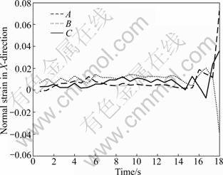
Fig.4 Normal strain with time in X-direction for three points

Figure 5 presents the change of the strains ε_X with time at point A. It can be seen from Fig.5 that the tensile strain at this point approaches to the local maximum at around 5.5 s, then decreases gradually with time as the cracks propagate, and increases rapidly after 15.5 s.

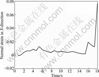
Fig.5 Normal strain with time in X-direction for point A

Figure 6 presents the changes of the normal strains ε_Y with time in the Y-direction for the points A, B, and C. It can be seen that the normal strain ε_Y has few changes between 1.0 and 11.0 s; ε_Y increases with a relatively large range between 14.0 and 16.0 s. After 16.0 s, there are relatively large changes in the behaviors and range of the normal strain at the point A, the tensile strain enlarges at a short interval followed by a gradual change at the point B, and a compressive strain continues at the point C. At 18.0 s, the specimen is in a failure status, and there are relatively small strains at the points A and B, while the compressive strain is relatively large at the point C.

Fig.6 Normal strain with time in Y direction for three points

From Figs.4-6, it can be seen that the normal strains are dependant on the locations and the crack distributions. Between 1.0 and 5.0 s prior to the specimen failure, normal strains increase rapidly at many locations, while a stable status appears at some locations.

Figure 7 presents the changes of the shear strains γ_XY with time at the points A, B, and C. It can be seen that the shear strains do not occur obviously before the previous 10.0 s. The shear strain γ_XY then increases gradually as the external loads increase. Between 15.0 and 18.0 s, γ_XY changes rapidly. When the specimen is in a failure  status at 18.0 s, there is a large γ_XY as increased in the inverse direction, implying that the clockwise rotation occurs.

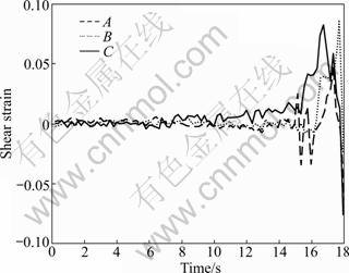
Fig.7 Shear strain with time

Figure 8 presents the contour map of the strain field of the specimen at 0.4 and 6.4 s. It can be seen that the normal strain ε_X is unevenly distributed at 0.4 s; the left and right parts of the specimen are respectively subjected to the compressive and tensile stresses. This agrees with the fact that the right part of the specimen has the original cracks and failure at first. Several strain concentration bands exist in Fig.8. As compared with the appearances in the specimen surface, it can be inferred that all of the bands do not completely develop into large cracks, while meso-cracks do not exist in some bands.

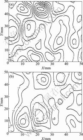
Fig.8 Contour maps of normal strain fields (10^-3): (a) At 0.4 s; (b) At 6.4 s

4 Conclusions

1) Using the video images taken in the uniaxial compression test of a limestone, the full-field displacements and strains at arbitrary time are obtained on the surface of the specimens.

2) In computing the displacements, the pattern matching technique and grayscale images are utilized. The application of filtering and iteration are also used to solve the problems involving in the selection of the window size in the matching algorithm. However, many factors, such as the instabilities of the surroundings and illuminants, and the noises in photographing, errors in computations, may influence the accuracy of the displacements. In addition, the matching requires much CPU-consumption. The image behaviors, such as the invariant momentum and fractal dimension, may be used as the features to perform the feature-based matching in the further study.

3)      In computing the strain, the number of the local displacements is a key value in using the least square method. If the number is too large, the full-fields may be relatively smooth and the estimated strains may be different from the true ones. However, if the number is too small, the full-fields may not be smooth and the noises may not be eliminated. In the current study, the number of the local displacements is selected as 5. Nevertheless, the determination of this number needs to be further examined. In the interpolation for the computation of the sub-pixel displacements, other methods, such as Lagrange and spline interpolations, may be used as the alternatives.

4)      From the full-field strain obtained in this study, it is found that the normal strains are dependant on the locations and the crack distributions as time passes. Between 1.0 and 5.0 s prior to the specimen failure, normal strains increase rapidly at many locations, while a stable status appears at some locations. Although several strain concentrations occur in the specimen, only a few of them develope into the visible cracks, resulting in the complete failure of the specimen.

5) The method proposed herein improves the traditional method for measuring the strain field. This improvement may be of great significance in investigating the deformation and/or failure mechanism of rock materials.

References

[1] DEB D, HARIHARAN S, RAO U M, RYU C H. Automatic detection and analysis of discontinuity geometry of rock mass from digital images [J]. Computers and Geosciences, 2008, 34: 115-126.

[2] XU J, ZHAO X, LIU B. Digital image analysis of fluid inclusions [J].International Journal of Rock and Mechanics Mining Sciences, 2007, 44(6): 942-947.

[3] YIN Xiao-tao, DANG Fa-ning, DING Wei-hua, CHEN Hou-qun. Morphologic measurement of crack in CT images of rock and soil [J]. Chinese Journal of Rock Mechanics and Engineering, 2006, 25(3): 539-544. (in Chinese)

[4] ZHAO Yong-hong, LIANG Hai-hua, XIONG Chun-yang, FANG Jing. Deformation measurement of rock damage by digital image correlation method [J]. Chinese Journal of Rock Mechanics and Engineering, 2002, 21(1): 73-76. (in Chinese)

[5] XU Jin-ming, WANG Qiang, ZHOU Ting-wen. Displacement field of limestone using video images from laboratory tests [J]. HydroGeology and Engineering Geology, 2010, 37(2): 70-75. (in Chinese)

[6] WANG Xue-qin, FAN Hong-li, WANG Yong. The application of model recognition in measuring strain-field of deforming sheet [J]. Journal of Hebei Institute of Technology, 2003, 25(2): 31-36. (in Chinese)

[7] CHEN Yin-li, YU Wei, HUANG Xiu-sheng. Application of digital image processing for strain analysis by square grid method [J]. Journal of Plasticity Engineering, 2009, 16(3): 182-186. (in Chinese)

[8] SHAO Long-tan, SUN Yi-zhen, WANG Zhu-pin, LIU Yong-lu. Application of digital image processing technique to triaxial test in soil mechanics [J]. Rock and Soil Mechanics, 2006, 27(1): 29-34. (in Chinese)

[9] WANG Feng, DAI Fu-long, XIE Hui-min, YING Hua. Measurement of strain factor of composites plate using moire interferometry [J]. Acta Mechanica Sinica, 1997, 29(5): 636-640. (in Chinese)

[10] ADAM J, URAI J L, WIENEKE B, ONCKEN O, PFEIFFER K, KUKOWSKI N, LOHRMANN J, HOTH S, ZEE W, SCHMATZ J. Shear localisation and strain distribution during tectonic faulting—New insights from granular-flow experiments and high-resolution optical image correlation techniques [J]. Journal of Structural Geology, 2005, 27: 283-301.

[11] CASTELLUCCIO G M, BRAVO R E, ERNST H A, YAWNY A A, PEREZIPI?A J E P. Simple application of open source PIV technique for measuring displacements and strains [C]// ALBERTO C, STORTI M, ZUPPA C. Mecánica Computacional XXVII. 2008: 1193-1203.

[12] WOLF H, K?NIG D, TRIANTAFYLLIDIS T. Experimental investigation of shear band patterns in granular material [J]. Journal of Structural Geology, 2003: 1229-1240.

[13] NIEDOSTATKIEWICZ M, LESNIEWSKA D, TEJCHMAN J. Experimental analysis of shear zone patterns in cohesionless for earth pressure problems using particle image velocimetry [J]. Strain: An International Journal for Experimental Mechanics, 2010, 46: 1-14.

[14] WHITE D J, TAKE W A, BOLTON, M D. Soil deformation measurement using particle image velocimetry (PIV) and photogrammetry [J]. Géotechnique, 2003, 53(7): 619-631.

[15] BHANDARI A R, INOUEN J. Strain localization in soft rock—A typical rate-dependent solid: experimental and numerical studies [J]. International Journal for Numerical and Analytical Methods in Geomechanics, 2005, 29: 1087-1107.

[16] ZHANG G, LIANG D, ZHANG J. Image analysis measurement of soil particle movement during a soil–structure interface test [J]. Computers and Geotechnics, 2006, 33: 248-259.

(Edited by YANG Bing)

Foundation item: Project(40972191) supported by the National Natural Science Foundation of China; Project(09YZ39) supported by the Creative Issue of Shanghai Education Committee, China

Received date: 2010-09-15; Accepted date: 2011-02-11

Corresponding author: XU Jin-ming, Professor, PhD; Tel: +86-21-56331972; E-mail: xjming@shu.edu.cn