
J. Cent. South Univ. Technol. (2007)05-0713-06
DOI: 10.1007/s11771-007-0136-7 ![]()
A new grey forecasting model based on BP neural network and Markov chain
LI Cun-bin(����), WANG Ke-cheng(�����)
(School of Business Administration, North China Electric Power University, Beijing 102206, China)
Abstract:
A new grey forecasting model based on BP neural network and Markov chain was proposed. In order to combine the grey forecasting model with neural network, an important theorem that the grey differential equation is equivalent to the time response model, was proved by analyzing the features of grey forecasting model(GM(1,1)). Based on this, the differential equation parameters were included in the network when the BP neural network was constructed, and the neural network was trained by extracting samples from grey system��s known data. When BP network was converged, the whitened grey differential equation parameters were extracted and then the grey neural network forecasting model (GNNM(1,1)) was built. In order to reduce stochastic phenomenon in GNNM(1,1), the state transition probability between two states was defined and the Markov transition matrix was established by building the residual sequences between grey forecasting and actual value. Thus, the new grey forecasting model(MNNGM(1,1)) was proposed by combining Markov chain with GNNM(1,1). Based on the above discussion, three different approaches were put forward for forecasting China electricity demands. By comparing GM(1, 1) and GNNM(1,1) with the proposed model, the results indicate that the absolute mean error of MNNGM(1,1) is about 0.4 times of GNNM(1,1) and 0.2 times of GM(1,1), and the mean square error of MNNGM(1,1) is about 0.25 times of GNNM(1,1) and 0.1 times of GM(1,1).
Key words:
grey forecasting model; neural network; Markov chain; electricity demand forecasting��
1 Introduction
Energy demand forecasting is very important to formulate energy policy of country, especially for those countries whose energy demand is growing quickly. With the rapid development of China��s economy, energy demand is surging, especially for the electricity demand. Accurately forecast electricity demand is the basis of economic planning, which is important not only for the electricity sectors, but also for the consumers.
Because there are numerous uncertainties in the electricity demand forecasting, these factors have determined that electricity demand forecasting is a complex process. To overcome this problem, DENG[1] proposed the grey forecasting model to study the system development tendency by using only few previous data. In recent years, the grey forecasting model has also been successfully employed in various fields such as traffic[2-3], electric power[4-6], chemistry[7] and satisfactory results have been obtained.
Although grey forecasting model has been widely adopted, its forecasting performance must be improved. The grey forecasting model is composed of exponential function[8-9]. For being infected by various random factors, the predictive accuracy and anti-jamming ability of grey forecasting model were reduced. To improve forecast accuracy and meet the actual demand, a new grey forecasting model based on BP neural network and Markov chain (MNNGM(1,1)) was proposed. Moreover, the proposed model was applied to forecating the electricity demand.
2 Traditional grey forecasting model GM(1,1)
The most commonly used grey forecasting model GM(1,1) consists of a single variable, and a first-order differential equation is adopted to match the data generated by the technique of accumulation generating operations(AGOs). For multi-variables grey forecasting model GM(1,N), its basic principle is the same as that of GM(1,1). GM(1,1) is the major research object for this research. The algorithm of GM(1,1) can be expressed as follows.
1) Listing the sequence corresponding to system variables.
![]()
2) Establishing the one-time AGO sequence:
![]()
![]() =
=
![]()
![]()
3) Establishing the grey differential equation:
![]()
This is a one-order one-variable differential equation model, so it is called GM(1,1), where a is the developing coefficient and b is the grey input.
4) Solving this equation parameter approximation (whitened value).
The above equation parameter vector is ![]() . The values of parameters can be estimated by the least-squares error method as
. The values of parameters can be estimated by the least-squares error method as
![]()
where

![]()
5) Getting the time response function of GM(1,1).
When x changes slowly, the interval unchanged value can be calculated for time response function. The approximate relationship on time of ![]() is presented as follows:
is presented as follows:
![]()
![]()
6) Predicting the value of x(0)(k+1).
The predicted value of x(0)(k+1) can be estimated as
![]()
3 New grey forecasting model based on neural network and Markov chain (MNNGM(1,1))
From the above algorithm GM(1,1) it can be found that changing sequence of numbers into differential equation model is the purpose of grey system model. Therefore a BP neural network can be constructed to whiten the grey differential equation. The differential equation parameters can be included in the network when the BP neural network is constructed. Extracted samples from the known data of grey system are used to train BP neural network. When BP network converges, the whitened grey differential equation parameters will be extracted. Thus, the accuracy and determined differential equation can be established and continuous system model can be achieved to increase the forecasting precision.
Moreover, there are a lot of stochastic phenomena in the process of the system development, the existence of these phenomenon reduces the accuracy of the grey forecasting model. However, Markov chain can be used to explain the stochastic phenomenon[10-11]. Grey forecasting model combined with Markov chain can reduce the random factor effects with the right model, thus it greatly reduces the stochastic effects of grey forecasting model.
3.1 Establishing the grey neural network forcasting model GNNM(1,1)
1) Using BP neural network to improve GM(1,1) and establish GNNM(1,1).
In order to facilitate the presentation, the grey symbols were changed as follows. The original sequence ![]() can be expressed as x(t), one-time AGO sequence
can be expressed as x(t), one-time AGO sequence ![]() can be expressed as y(t), the forecasting value
can be expressed as y(t), the forecasting value ![]() can be expressed as z(t), where t��(0, N-1).
can be expressed as z(t), where t��(0, N-1).
Theorem 1 The grey differential equation is equivalent to the time response model.
Proof The following proves the validity of GM(1,1).
In grey system, grey differential equation GM(1,1) can be expressed in the following form:
![]() (1)
(1)
According to previous statements, Eqn.(1) can be expressed in the following form:
![]() (2)
(2)
where a and u are the pending parameters. The time response model is:
![]() (3)
(3)
The discrete response model is
![]() (4)
(4)
Moreover, the grey differential equation ![]() can be solved in the following expression:
can be solved in the following expression:
![]() (5)
(5)
When t=0, y(0)=x(0), then ![]() . And
. And
![]() (6)
(6)
Thus, the theorem is proved. Similarly, the same conclusion is applied to GM(1, N).
In light of these conclusions, the use of time response model based on neural network is more reasonable. Eqn.(3) is transformed as follows. It is mapped to a BP neural network, and then trains the BP neural network. When network converges, the corresponding equation coefficients are extracted from the BP neural network. Thus, an whitened equation can be established, and this equation for further research can be used or can be solved.
Eqn.(3) is transformed as follows:
![]() =
=![]() =
=
![]() (7)
(7)
According to Eqn.(7), the structure of BP neural network is shown in Fig.1.
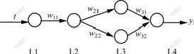
Fig.1 Structure of BP neural network structure
Then, the corresponding BP network weights can be assigned as follows:
 (8)
(8)
The threshold of ![]() can be expressed as
can be expressed as
![]() (9)
(9)
Neuron activation function of BP neural network of layer L2 can be chosen as Sigmoid function: ![]() Other layers�� activation function is f(x)=x.
Other layers�� activation function is f(x)=x.
Through neural network training, weights can be corrected repeatedly, equivalent to the whitened parameters constant, thereby enhancing the accuracy of forecasting. Thus, grey neural network model GNNM(1,1) is proposed.
2) Learning algorithm of GNNM (1,1).
As grey BP neural network is different from the traditional BP neural network, the learning algorithm of traditional BP neural network will be improved to adapt grey BP neural network.
There are two points need to be paid attention when grey BP neural network is trained. On one side, because w21=-y(0) , w21 remains unchanged in training BP neural network. On the other side, w31 and w32 can be calculated by input data and w11. Specific learning algorithm can be stated as follows.
Step 1 According to the system��s sequence features, selecting two smaller values a and u.
Step 2 According to network weights definition, calculating w11, w11*,w21, w22*,w22, w31 and w32, where w11* and w22* are weights of w11 and w22, respectively, after being adjusted.
Step 3 For each mode(t, y(t)) (t=1, 2, 3, ��, N) , the procedure applied are as follows.
Step 3.1 Feeding input to layer L1 nodes and calculating the nodes of layers L2, L3 and L4.
Layer L2: ![]() .
.
Layer L3: c1=bw21, c2=aw22.
Layer L4: d=w31c1+w32c2.
Step 3.2 Calculating the error of network output and desiring output.
As layer L4 activation function is f(x)=x, f ��(x)=1, the error of layer L4 is
![]() (10)
(10)
The error is reversely transferred to layer L3, layer L3 activation function is f(x)=x, the error of layer L3 is
![]() (11)
(11)
Reversely, transferring of layer L3 error to that of layer L2, for layer L2 the activation function is ![]() , the error of layer L2 is
, the error of layer L2 is
![]() =
=
![]() =
=
![]() (12)
(12)
Step 3.3 Adjusting the connection weights from layer L2 to layer L3.
w22*=w22-�̦�2b (13)
Step 3.4 Adjusting the connection weights from layer L1 to layer L2.
w11*=w11-����2t (14)
Step 3.5 Adjusting threshold.
For ![]() , w22=b, the adjustment threshold of layer L4 is as follows:
, w22=b, the adjustment threshold of layer L4 is as follows:
![]() (15)
(15)
Step 4 Repeating step 3 until the error approaches to 0 or satisfies the necessary requirements.
3.2 Establishing new grey model MNNGM(1,1) by combining GNNM(1,1) with Markov chain
Using Markov chain to improve GNNM(1,1) and establish the proposed grey forecasting model MNNGM(1,1), the specific process is as follows.
As there are residual sequences between grey forecasting and actual values, the size and characteristics of residual sequences are used to express the influence of the stochastic phenomenon. Based on original sequences x(0), forecast is made on the series ![]() , then the residual sequences between them is
, then the residual sequences between them is
![]() ��,
��,![]() (16)
(16)
were ![]() ��k=2, 3, ��, n.
��k=2, 3, ��, n.
Markov transition matrix can provide the expectations of the possible correction for the prediction of the value for the next step. To conduct Markov state transition matrix, states are defined for each time step. Each state has an interval whose width is equal to a fixed portion between the maximum and the minimum of the whole residual errors. Then the state of the transmission probability can easily be defined. The state transition probability from state i to state j after m steps is stated as follows:
![]() ��
�� ![]() =1, 2, ��, s (17)
=1, 2, ��, s (17)
where ![]() is the number of state transition from state i to state j after m steps and Mi is the total number of state i. Finally, the s-state m-step state transition matrix is defined as
is the number of state transition from state i to state j after m steps and Mi is the total number of state i. Finally, the s-state m-step state transition matrix is defined as
 (18)
(18)
The arbitrary state of the transfer matrix can be obtained according to Eqn.(16), through the analysis of trends and patterns of transmission probability, the probability of the next state can be predicted. Defining the centers of each state as vi(i=1, 2��, s) and the possibility of each transition state as wi(i=1,2, ��, s), then, the next step predictive value is stated as follows:
![]() (19)
(19)
where ��i is the corresponding weight for the state i. Usually, ��i can be estimated as[12]: ![]() Therefore, the predicted values of GNNM(1,1) can be amended as follows:
Therefore, the predicted values of GNNM(1,1) can be amended as follows:
![]() (20)
(20)
Through the above analysis, MNNGM(1,1) is finally established by combining Markov chain with GNNM(1,1). On one hand, the prediction accuracy are enhanced, on the other hand, the influence of stochastic phenomenon for forecasting values is reduced, thus the system forecasting accuracy is improved.
4 Example analysis
To demonstrate the effectiveness and accuracy of the proposed grey forecasting model, GM (1,1), GNNM (1,1), MNNGM (1,1) were applied to China electricity demand forecast, respectively. The data were collected from China Statistical Annual[12]. The three models were used to forecast and analyze China electricity demand during 1990-1998��s to compare the effectiveness of each model, as well as the difference accuracy of forecasting, while the 1999-2001 data were used as testing data set.
In order to compare the difference accuracy of three model forecasting, three evaluation criteria were used[13]: the relative error (ER), the mean square error (EMS), and the absolute mean error (EAM). The formula for ER is
![]() (21)
(21)
where x(k) is the actual value at time k and ![]() is the predicted value. The formula for EMS is
is the predicted value. The formula for EMS is
![]() (22)
(22)
where n is the number of data used for forecasting. The formula for EAM is
![]() (23)
(23)
Based on the above analysis of GM (1,1), GNNM (1,1) and MNNGM (1,1), the three models were built and the relative error were analyzed according to data during 1990-1998, where using 1990-1998��s data as model building data set and 1999-2001��s data as ex-post testing set. The observed and forecasted values are shown in Table 1 to compare the three model��s accuracy and relative error. Using data in 1999-2001 as data set to compare the three models�� accuracy and relative error. The corresponding calculated results are shown in Table 2.
From Table 1 it can be seen that three models present quite satisfactory forecasting results. By comparing the relative error, the relative error of GNNM(1,1) is smaller than that of GM(1,1). For BP neural, the improved network GM(1,1) and the convergence rate have more precise prediction. Moreover, MNNGM(1,1) has higher precise prediction than GNNM(1,1).
Table 3 shows EMS and EAM of the three models. It can be seen from Table 2 that MNNGM (1,1) has higher forecasting accuracy according to different criteria. For example, in 1999-2001, EAM of MNNGM(1,1) is about 0.4 times of GNNM(1,1) and 0.2 times of GM(1,1). In other words, the forecasting accuracy of MNNGM(1,1) is about 2.5 times of GNNM(1,1) and 5 times of GM(1,1) for China electricity demand. While EMS of MNNGM(1,1) is about 0.25 times of GNNM(1,1) and 0.1 times of GM(1,1). This proves the effectiveness and accuracy of MNNGM(1,1) algorithm.
Figs.2-4 show the forecasting results of the three models respectively. From Fig.2 it can be seen that although GM(1,1) has the better forecasting precision in 1990-1996, the accuracy starts to decline obviously after 1996. In Fig.3, the forecasting curve of GNNM(1,1) is more close to observed curve than the curve of GM(1,1), especially the forecasted value after 1998. From Fig.4 it can be seen that MNNGM(1,1) has the highest forecasting accuracy.
Table 1 Observed and forecasted electricity demands during 1990-2001 using three different approaches in China
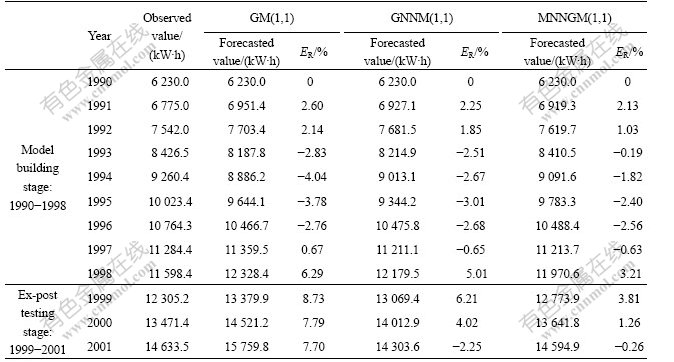
Table 2 Error analytical results of different forecasted models
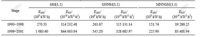
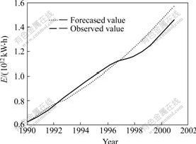
Fig.2 Forecasting results of GM(1,1)
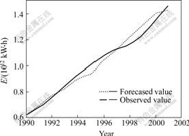
Fig.3 Forecasting results of GNNM(1,1)
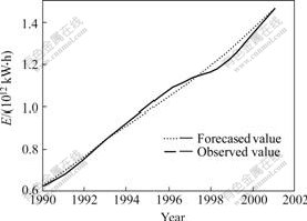
Fig.4 Forecasting results of MNNGM(1,1)
5 Conclusions
1) The grey neural network forecast model is built by combining grey forecasting model with neural network, which expands the application scope of GM(1,1) and improves the forecasting precision.
2) The grey differential equation is equivalent to the time response model is proved, which provides the foundation for combining grey forecasting model with BP neural network. Moreover, the corresponding learning algorithm is proposed.
3) To build the proposed grey forecasting model MNNGM(1,1), GNNM(1,1) is improved by using Markov chain. Considering the random factors, the proposed model has more realistic applications.
4) Other than the stochastic phenomenon of grey forecast model, there exist some periodic phenomena. The future work is to improve this problem and enhance the model��s robustness.
References
[1] DENG Ju-long. Control problem of grey system[J]. System and Control Letters, 1982, 1(5): 288�C294. (in Chinese)
[2] WU Da-zhi, LI Xi-bing, JING Wei-dong. Application of grey theory to the settlement prediction for high fills[J]. Journal of Central South University of Technology: Science and Technology, 2002, 33(3): 230-233. (in Chinese)
[3] ZHANG Fei-lian, SHI Feng. Stochastic grey system model for forecasting passenger and freight railway volume[J]. Journal of Central South University: Science and Technology, 2005, 36(1): 158-162. (in Chinese)
[4] AKAY D, ATAK M. Grey prediction with rolling mechanism for electricity demand forecasting of Turkey[J]. Energy, 2007, 32(9): 1670�C1675.
[5] ZHOU P, ANG B W, POH K L. A trigonometric grey prediction approach to forecasting electricity demand[J]. Energy, 2006, 31(14): 2839�C2847.
[6] WANG Jian-zhou, MA Zhi-xin, LI Lian. Detection, mining and forecasting of impact load in power load forecasting[J]. Applied Mathematics and Computation, 2005, 168(1): 29�C39.
[7] PAI T Y, TSAI Y P, LO H M, et al. Grey and neural network prediction of suspended solids and chemical oxygen demand in hospital wastewater treatment plant effluent[J]. Computers and Chemical Engineering, 2007, 31(10): 1272�C1281.
[8] DENG Ju-long. The Theory Book of Grey System[M]. Wuhan: Huazhong University of Science and Technolog Press, 1990. (in Chinese)
[9] YE Ming-quan, HU Xue-gang. Seasonal artificial neural network forecasting model and its applicaiotn in the GM(1,1) residual error correcation[J]. Computer Engineering and Applications, 2005, 4(1): 194-196. (in Chinese)
[10] HSU L C, WANG C H. Forecasting the output of integrated circuit industry using a grey model improved by the Bayesian analysis[J]. Technological Forecasting & Social Change, 2007, 74(6): 843-853.
[11] MEYN S P, TWEEDIE R L. Markov Chains and Stochastic Stability[M]. New York: Springer�CVerlag, 1993.
[12] National Bureau of Statistics of China (various years). China Statistical Yearbook[M]. Beijing: China Statistical Press. (in Chinese)
[13] LIN Yong-huang, LEE P C. Novel high-precision grey forecasting model[J]. Automation in Construction, 2007, 16(6): 771�C777.
Foundation item: Project(70572090) supported by the National Natural Science Foundation of China
Received date: 2007-03-20; Accepted date: 2007-05-18
Corresponding author: LI Cun-bin, Professor; Tel: +86-10-51963787; E-mail: lcb999@263.net
(Edited by CHEN Can-hua)
Abstract: A new grey forecasting model based on BP neural network and Markov chain was proposed. In order to combine the grey forecasting model with neural network, an important theorem that the grey differential equation is equivalent to the time response model, was proved by analyzing the features of grey forecasting model(GM(1,1)). Based on this, the differential equation parameters were included in the network when the BP neural network was constructed, and the neural network was trained by extracting samples from grey system��s known data. When BP network was converged, the whitened grey differential equation parameters were extracted and then the grey neural network forecasting model (GNNM(1,1)) was built. In order to reduce stochastic phenomenon in GNNM(1,1), the state transition probability between two states was defined and the Markov transition matrix was established by building the residual sequences between grey forecasting and actual value. Thus, the new grey forecasting model(MNNGM(1,1)) was proposed by combining Markov chain with GNNM(1,1). Based on the above discussion, three different approaches were put forward for forecasting China electricity demands. By comparing GM(1, 1) and GNNM(1,1) with the proposed model, the results indicate that the absolute mean error of MNNGM(1,1) is about 0.4 times of GNNM(1,1) and 0.2 times of GM(1,1), and the mean square error of MNNGM(1,1) is about 0.25 times of GNNM(1,1) and 0.1 times of GM(1,1).
