
J. Cent. South Univ. (2016) 23: 2465-2474
DOI: 10.1007/s11771-016-3305-8

Cumulative prospect theory-based user equilibrium model with stochastic perception errors
WANG Wei(��ΰ), SUN Hui-jun(����)
Key Laboratory of Urban Transportation Complex Systems Theory and Technology of Ministry of Education, Beijing Jiaotong University, Beijing 100044, China
 Central South University Press and Springer-Verlag Berlin Heidelberg 2016
Abstract:
The cumulative prospect theory (CPT) is applied to study travelers�� route choice behavior in a degradable transport network. A cumulative prospect theory-based user equilibrium (CPT-UE) model considering stochastic perception error (SPE) within travelers�� route choice decision process is developed. The SPE is conditionally dependent on the actual travel time distribution, which is different from the deterministic perception error used in the traditional logit-based stochastic user equilibrium. The CPT-UE model is formulated as a variational inequality problem and solved by a heuristic solution algorithm. Numerical examples are provided to illustrate the application of the proposed model and efficiency of the solution algorithm. The effects of SPE on the reference point determination, cumulative prospect value estimation, route choice decision and network performance evaluation are investigated.
Key words:
cumulative prospect theory; user equilibrium; stochastic perception error; variational inequality��
1 Introduction
Given that the cumulative prospect theory (CPT) provides a well-supported descriptive paradigm for decision making under risk or uncertainty, many studies applied the theory to model travelers�� route choice behavior in stochastic transport network and developed CPT-based user equilibrium models. AVINERI [1] investigated the effect of reference point (RP) value on the stochastic network equilibrium based on CPT. CONNORS and SUMALEE [2] proposed a general CPT-based user equilibrium (CPT-UE) model for stochastic networks. SUMALEE et al [3] studied CPT-UE model in a network where demand and supply uncertainties are considered endogenously. XU et al [4] presented a multiclass CPT-UE model with endogenous RP for stochastic networks. TIAN et al [5] developed a CPT-based dynamic user equilibrium (CPT-DUE) model by applying the CPT to formulate the travelers�� risk evaluation on arrival time. YANG and JIANG [6] employed the cumulative prospect value (CPV) to replace the utility value in the logit model and proposed a stochastic user equilibrium model based on CPT (CPT-SUE). XU et al [7] also used the CPT-SUE approach to model road user behavioral changes over time.
An assumption that pervades the literature above is that the actual probability distributions of the random travel time are assumed to be known exactly to travelers. However, due to the imperfect knowledge about the network condition, travelers�� perception errors should be incorporated into their decision process. The traditional SUE model considers the kind of perception error which is regarded as ��deterministic��, because it is independent of the stochastic travel time. However, MIRCHANDANI and SOROUSH [8] stated that the deterministic perception error may not well reflect travelers�� perception on the travel time distribution (TTD). They suggested using a stochastic perception error (SPE), which is conditional on the actual TTD and different from the deterministic perception error used in the traditional logit model. In that case, incorporating the SPE into the actual TTD forms the perceived TTD. This can be illustrated in Fig. 1. Consequently, travelers should make route choice decisions based on the perceived TTD rather than the actual one [9-10]. Therefore, in the CPT-based route choice model, it is reasonable to assume that travelers make their decisions based on the perceived TTD rather than the actual one. Due to the differences between the actual TTD and the perceived TTD, the travelers�� route choice decisions could be quite different.
In this work, the traditional CPT-UE model is extended by explicitly modeling the SPE within the travelers�� route choice decision processes. Several features distinguish this work from those found in the literature. First of all, travelers are assumed to determine their endogenous reference time points based on the perceived TTD rather than the actual one. Then, the CPVs of all paths for each O-D pair are calculated by the perceived TTD rather than the actual one. Thirdly, the effects of SPE in the CPT-UE model on the travelers�� route choice behavior (in terms of equilibrium flows and CPVs) and network performance (in terms of the total TTD) are examined, which seems not to have been studied before. Finally, in order to enhance the understanding of the effect of SPE and also the visualization on perceived TTD, the distribution fitting method is used to estimate the probability distribution of stochastic travel time.
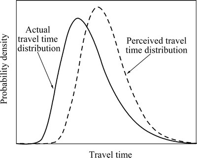
Fig. 1 Illustration of actual and perceived travel time distributions
2 Travel time distribution
2.1 Notations and assumptions
The notations used in this work are listed in Nomenclature.
To facilitate the presentation of the essential ideas without loss of generality, the following basic assumptions are made.
Assumption 1: The link capacity is independent of the amount of traffic on it.
Assumption 2: The link travel time is independent from each other.
Assumption 3: Travelers�� perception errors are independent for non-overlapping route segments.
Assumption 4: Travelers�� perception errors are mutually independent over the population of travelers.
2.2 Actual travel time distribution
To model congestion, let us consider the widely adopted Bureau of Public Road (BPR) link travel time function:
 (1)
(1)
where  and
and  are the deterministic parameters in BPR function. Assuming that the link capacity Ca follows a uniform distribution defined by an upper bound (the design capacity
  and a lower bound (the worst-degraded capacity). According to Refs. [11-12], the lower bound is assumed to be a fraction
  of the design capacity. Then, the nth moment of 1/Ca can be derived as
 (2)
(2)
Using the binomial expansion, the nth moment of the actual link travel timecan be derived as follows [9]:
 (3)
(3)
Thus, the actual route travel time variable can be expressed by summing the corresponding link travel time variables as
 (4)
(4)
2.3 Perceived travel time distribution
Definition 1: The stochastic perception error  for link a is conditional on the stochastic link travel time Ta and normally distributed as [9-10]
 (5)
(5)
According to Eq. (5), the stochastic perception error distribution of an individual traveler for a segment of road with a unit travel time is  where
where  denotes a normal distribution with mean �� and variance ��2. The parameters �� and ��2 are predefined and deterministic.
Definition 2: The perceived travel time  on route k between O-D pair r is defined as the sum of the actual travel time
  and the SPE
  which is conditional on the stochastic route travel time, and the following equation is satisfied [9-10] as

 (6)
(6)
A detailed derivation of the probability distribution statistics for the perceived link and route travel time variables is provided in Appendix A.
2.4 Fitting route travel time distribution by moments
HILL et al [13] proposed a numerical method that makes use of the first four moments of a random variable to match any distribution in the Johnson curve system. CLARK and WATLING [14] adopted the same method to estimate the full distribution of total travel time. In this section, a numerical method is described to estimate the whole perceived route travel time distribution. Empirical study revealed that route travel time distribution is typically asymmetric with a long and fat tail. Therefore, the lognormal distribution is used to estimate the probability distribution of perceived route travel time.
Consider the following lognormal random variable X by
 (7)
(7)
where Z is a standard normal variable, i.e. Z~N(0,1), and  , ��, and �� are parameters. Then, the probability density function (PDF) of X is as

 (8)
(8)
The remaining work is to calculate the values of the three parameters. First, the following equation is solved to obtain ��
 (9)
(9)
The three parameters in Eq. (7) can then be calculated as

 (10)
(10)
After calibrating the above parameters, the fPDF in Eq. (8) is actually known. Then, an estimated distribution of the random variable X can be obtained. As a consequence, the fPDF of the perceived route travel time can be obtained using the distribution fitting method discussed above.
3 Cumulative prospect theory
Given that CPT provides a well-supported descriptive paradigm for individuals�� decision making under risk or uncertainty, the CPTis adopted to describe travelers�� route choice behavior in this section.
3.1 Value function
Considering a trip between O-D pair r with ��r as the RP for the drivers. Compared to the RP, travelers may consider the outcome of a trip as a gain, if the travel time is less than the RP; as a loss if otherwise. The canonical example of a value function gr(x) is
 (11)
(11)
where x denotes the perceived route travel time; parameters �� and �� measure the degree of diminishing sensitivity of value function. Typically, 0 < ��, �� < 1 and thus the value function exhibits risk aversion over gains and risk seeking over losses. The parameter �� �� 1 is called ��loss-aversion�� coefficient, indicating the individuals are more sensitive to losses than gains.
3.2 Probability weighting function
Based on experimental evidence, CPT proposes that small probabilities are typically over-weighted, moderate and high probabilities are under-weighted. A typical inverse S-shaped probability weighting function is presented as
 (12)
(12)
where w(p) and p denote the decision weight and probability of an event respectively. The parameter �� represents the level of distortion in probability judgment in the decision making process and 0<��<1.
3.3 Reference points
XU et al [4] assumed that the RP for a traveler is the time he or she budgeted to ensure his or her desired on-time arrival probability. This time will depend on trip purpose and risk attitude. Mathematically, suppose that a traveler has a desired on-time arrival probability of ��r, the budgeted time for taking path k of O-D pair r, i.e. , can be written as
 (13)
(13)
With a continuous travel time distribution, taking the inverse of Eq. (13) leads to
 (14)
(14)
where is the inverse function of
It is assumed that the RP is the minimum of the budgeted times of all paths. that is,
 (15)
(15)
3.4 Cumulative prospect value
The CPV perceived by the drivers on route k between O-D pair r can be calculated as [2-4]

 (16)
(16)
where  and
and  are the lower and upper bounds of the perceived travel time on path k, respectively. In this work, the lower bound of the route travel time is assumed to be the free-flow travel time and the upper bound of the route travel time is assumed to be the 99.9999 percentile of the random travel time.
4 CPT-UE model and solution algorithm
4.1 CPT-UE model
Definition 3: The CPT-UEis a network state such that for each O-D pair, the CPVs of all used routes are equal, which are no less than the CPV of any unused route. No traveler can thus further increase his or her CPV by unilaterally changing routes. At equilibrium, travelers will stop adjusting their RPs, which remain constant and are consistent with the resulting CPT-UE flow pattern and the corresponding perceived TTDs.
The above descriptive definition can be mathematically represented as
 (17)
(17)
where ��r is the maximum TPV between O-D pair r, i.e.  .
.
Then, the CPT-UE conditions can be equivalently formulated as the following variational inequality (VI) problem, which is to find a route flow pattern  , such that
 (18)
(18)
where 

 denotes the constraint set that consists of the following equations:
 (19)
(19)
 (20)
(20)
 (21)
(21)
The following propositions give the equivalence of the VI formulation and the proposed CPT-UE model as well as the existence of the equilibrium solutions.
Proposition 1: The solution of the VI problem (Eq. (18)) is equivalent to the equilibrium solution of the CPT-UE model with SPE.
Proof: Equation (18) is equivalent to 
 Thus, f * is a solution to the VI problem (Eq. (18)) if and only if it is a solution to the following linear programming model with the same solution vectors (i.e. route flow):
 (22)
(22)
Using the relationship between the primal and dual solutions of linear programming (22), it follows that
 (23)
(23)
 (24)
(24)
Obviously, Eqs. (23) and (24) ensure that the equilibrium route flow pattern satisfies the CPT-UE conditions (Eq. (17)). This completes the proof.
Proposition 2: The CPT-UE model with SPE has at least one solution.
Proof: According to Proposition 1, the equivalent VI formulation is only needed to consider. Note that the feasible set �� is nonempty and convex. Furthermore, consider the link travel time function, value function and CPV function, it is reasonable to know that the mapping  is continuous. Thus, the VI problem (Eq. (18)) has at least one solution. This completes the proof. However, note that the solution to the VI problem is not unique in general. The reason is that the mapping in the VI formulation may be not strictly monotone due to the complicated function for the CPV.
4.2 Solution algorithm based on method of successive average
The method of successive average (MSA) can be adopted to solve the equilibrium assignment defined in Eq. (18) [3-4, 15]. The MSA algorithm is briefly described as follows.
Step 1: Initialization. Set l = 1 and specify an initial route flow pattern 
Step 2: CPV calculation. Calculate the CPV for each route, 
Step 3: Search direction finding. For each OD pair, find the route with the maximum CPV. Define an route flow pattern  with
with  if
if  and 0 otherwise.
Step 4: Check convergence. Evaluate 
 terminate the algorithm if
  or
or  where �� is the convergence criteria and lmax is the pre-set maximum number of iteration. The M(f (l)) is a convergence indicator measuring how closely a solution of the lth iteration satisfies the CPT-UE condition (Eq. (18)).
Step 5: Route flow updating. Update the route flow pattern as  where step size s(l)=1/l. Set l = l + 1, go to Step 2.
5 Numerical examples
To illustrate the proposed CPT-UE model with travelers�� SPE and solution algorithm, two networks are adopted in the numerical experiments. First, a small network is used to analyze the features of the proposed model and its difference compared to CPT-UE model without SPE. Then, the well-known Nguyen-Dupuis network is employed to demonstrate the applicability of the solution algorithm and the effects of the SPE on the network performance.
5.1 Small network
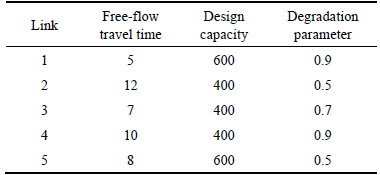
A simple network consists of four nodes, five links and three routes as shown in Fig. 2 is adopted. There is one OD pair (1,4) with 1000 units of demand. The free-flow travel time, design capacity and degradation parameter for each link are listed in Table 1. The convergence criterion and the maximum iteration number are set as �� = 0.25 and lmax=500.
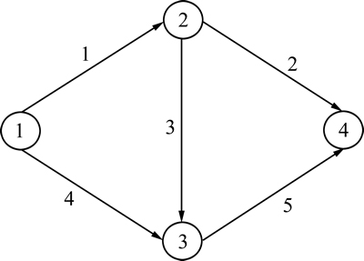
Fig. 2 Small network
Table 1 Network characteristics
It is assumed that the travelers are all risk averse and the desired on-time arrival probability is 80% and the perception error distribution of a unit travel time follows N(0.4,(0.4)2). The coefficients of the BPR function in Eq. (1) are  and
and  The parameters of the value function in Eq. (11) are assumed to be �� = 0.37, �� = 0.59, �� = 1.51, and the probability weighting function in Eq. (12) is used with �� = 0.74. The results of equilibrium path flows with and without SPE are presented in Table 2 and Fig. 3. The equilibrium result with SPE is shown by the bracketed figures in Table 2.
From Table 3 and Fig. 3, it can be seen that the equilibrium route flow pattern obtained from the model with SPE is significantly different from those obtained from the one without SPE. In particular, the differences can be explained by the following reason: travelers choose the reference time points and estimate CPV of each path based on the perceived and actual travel time distribution, respectively.
Table 2 Equilibrium route flow patternswith and without SPE
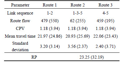

Fig. 3 Equilibrium route flow patterns with and without SPE
Table 3 Link-route incidence relationship
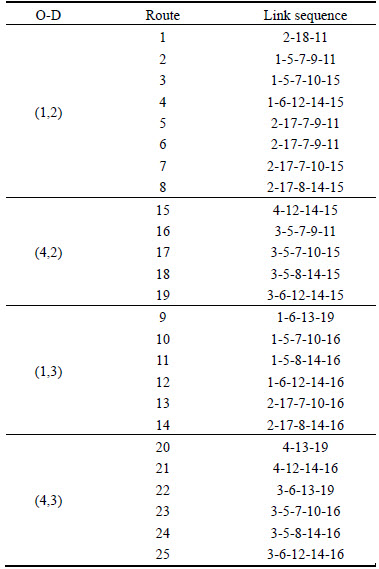
Figure 4 depicts the perceived and actual TTD could be significantly different for all the three routes. This discrepancy is attributed to the consideration of the SPE, which plays an important role in making route choice decisions under CPT-based behavioral assumption.
In order to further examine the effect of SPE on the perceived TTD, we set the SD at 0, 0.2 and 0.4, respectively. Their corresponding CDFs in route 1 are shown in Fig. 5. It is found that the perceived TTD gradually move to the right with a larger variability with the increase of SPE variance. This means that for a given cumulative probability (e.g., 80%), the perceived travel time is increasing with the SPE variance.
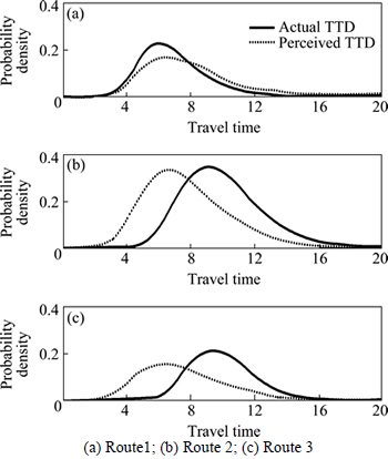
Fig. 4 Probability distribution of perceived and actual route travel times:
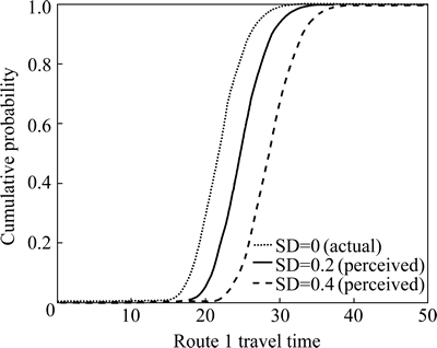
Fig. 5 Actual and perceived TTDs under different SPE variances
The impacts of SPE on the equilibrium RP and CPV are displayed in Figs. 6 and 7, respectively. From these figures, it can be seen that the RP and CPV increase as �� and �� increase. This is to be expected, because �� and �� of the perception error contribute to a larger variance of the perceived TTD. Therefore, in order to reach the specified travel time reliability requirement and also avoid unacceptable delay, higher RP is required and larger CPV is obtained.
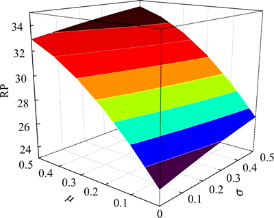
Fig. 6 Impact of SPE on RP
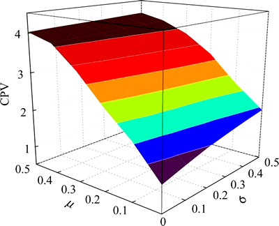
Fig. 7 Impact of SPE on CPV
5.2 Nguyen-dupuis network
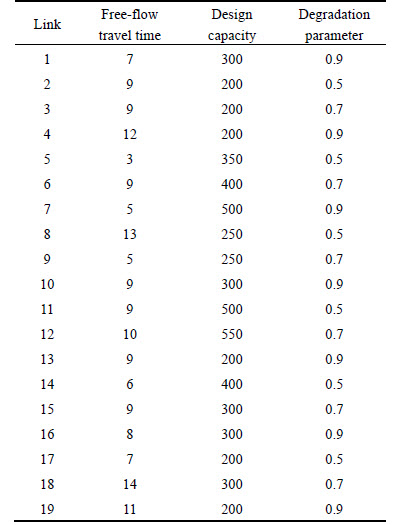
In this example, the well-known Nguyen-Dupuis network is used to further demonstrate the CPT-UE model and solution algorithm. The Nguyen-Dupuis network, shown in Fig. 8, contains 13 nodes, 19 directed links, 4 O-D pairs, and 25 routes. The link-route incidence relationship is shown in Table 3. The values of the base travel demands of O-D pairs (1, 2), (1, 3), (4, 2), and (4, 3) are 600, 500, 400, and 500, respectively. The free-flow travel time, design capacity and degradation parameter for each link are listed in Table 4. For simplicity, we further assume all travelers have the same confidence level of 80%. The parameters of the BPR function, the value function and the probability weighting function are the same as in the above example. The perception error is normally distributed with the mean of 0.5 and standard deviation of 0.5.
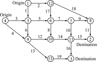
Fig. 8 Nguyen-dupuis network
Table 4 Link characteristics
The convergence characteristic of the solution algorithm is shown in Fig. 9. As can be seen, the algorithm terminates at iteration 347th given the convergence criteria that M is almost equal to zero. This illustrates that the proposed solution algorithm can converge to a stable solution for the medium-size network.
The impact of SPE on the mean of total travel time (TTT) is shown in Fig. 10. From this figure, it can be known that the TTT goes up as �� and �� increase.Figure 10 alsopresents that travelers�� SPE of travel time variability has a bad effect on the system performance. It is believed that the proposed model in this paper can be used to investigate the effects of advanced traveler information system (ATIS) with different travel time information.
The TTT distributions corresponding to the system optimal (SO), the CPT-UE model without SPE and the CPT-UE model with SPE are revealed in Fig. 11. It can be observed that: 1) The TTT distribution corresponding to the CPT-UE with SPE is obviously different from that corresponding to the CPT-UE without SPE. 2) The TTT distribution under the CPT-UE considering SPE has the largest variance and asymmetry. The large variance is due to the consideration of SPE, which adds extra uncertainty to the total travel time variability. 3) Considering travelers�� SPE on network conditions, the TTT becomes larger and more random. Therefore, ignoring the SPE in the CPT-UE models can lead to bias estimation of the TTT distribution, resulting in an inaccurate network performance assessment.
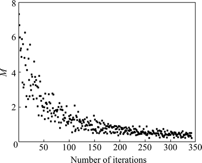
Fig. 9 Convergence of solution algorithm for Nguyen-Dupuis network
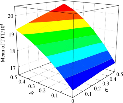
Fig. 10 Impact of SPE on TTT
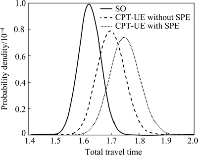
Fig. 11 Impact of SPE on TTT distribution
Figure 12 plots the sensitivity of the equilibrium CPV of OD pair (1-2) to changes in �� and �� at the RP (��r=80%). Similar tests at other OD pairs are carried out through not displayed here due to space limitations. For high values of RP (��r = 80%), the CPV is more sensitive to changes in �� (risk aversion to gain); the nature of risk seeking to loss (via ��) is limited since loss is rarely experienced. Figure 13 depicts the sensitivity of the equilibrium CPVs to the change in ��. �� determines the distortion of the probability perception in which as  the probability weighting function becomes identify mapping. From Fig. 13, as the CPVs of all OD pairs converge to a particular value which is indeed an average of the value function.
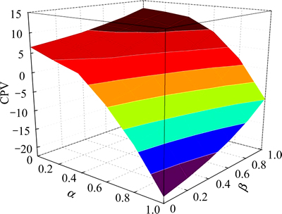
Fig. 12 Sensitivity analyses of �� and �� parameter values
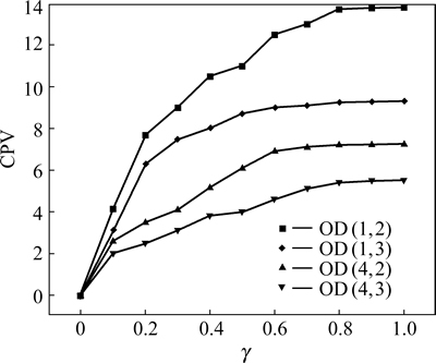
Fig. 13 Sensitivity analyses of �� parameter value
6 Conclusions
1) The traditional CPT-UE model is extended by explicitly modeling travelers�� SPE within their route choice decision processes. The SPE is conditionally dependent on the actual TTD, which is different from the deterministic perception error used in the traditional logit-type SUE models. Then, travelers will make route choice decision based on the perceived TTD rather than the actual one.
2) The CPT-UE model with SPE is formulated as a variational inequality problem and solved by a heuristic solution algorithm. Two numerical examples are provided to highlight the essential ideas of the proposed model and to demonstrate the solution algorithm. The numerical results indicate the importance of explicitly considering the SPE in the CPT-UE models. For the travelers, ignoring the SPE will affect their route choice and trip time planning. For the network planners, ignoring the SPE in the CPT-UE models can lead to bias estimation of equilibrium traffic flows and inaccurate assessment of network performance.
3) The effects of SPE in the CPT-UE model are investigated at four levels: the determination of reference time points for each O-D pair, the estimation of the probability distribution of route travel time and the calculation of CPV for each path, travelers�� route choice decision and user equilibrium pattern and network performance.
4) For future research, multiple user classes with various perception errors should be considered. In addition,it is interesting but challenging to present the application of the proposed CPT-UE model in congestion pricing and traffic network design.
Nomenclature
G=(N, A)
A road network, with N and A being sets of nodes and links respectively
R
Set of origin-destination (O-D) pairs
Kr
Set of routes for O-D pair 
qr
Total travel demand for O-D pair

Traffic flow on route  between O-D pair r
va
Traffic flow on link 
Ta
Actual travel time on link

Perceived travel time on link

Free-flow travel time on link
Ca
Capacity on link
Actual travel time on path
Perceived travel time on path

Indicator variable that is equal to 1 if path contains link, and 0 otherwise

CPV of path with perceived TTD

CDF of perceived travel time on path
Abbreviations
CPT
Cumulative prospect theory
CPT-UE
Cumulative prospect theory-based user equilibrium
CPT-SUE
Cumulative prospect theory-based stochastic user equilibrium
CPT-DUE
Cumulative prospect theory-based dynamic user equilibrium
RP
Reference point
CDF
Cumulative distribution function
Probability density function
CPV
Cumulative prospect value
TTT
Total travel time
SPE
Stochastic perception error
BPR
Bureau of Public Road
VI
Variational inequality
ATIS
Advanced traveler information system
SD
Standard deviation
Appendix A
The first to fourth origin moments of the perceived link TTD can be derived as follows:

 (25)
(25)


 (26)
(26)
Consequently, the second central moments of the perceived link TTD can be represented as follows:

 (27)
(27)
It is well known that the first to fourth cumulants of the perceived link TTD can be derived from the central moments as follows:

 (28)
(28)

 (29)
(29)
From the additive property of the cumulants, the first to fourth cumulants of the perceived route TTD can be obtained as follows:

 (30)
(30)
Denote  and
and  as the expected value and standard deviation (SD) of the perceived route travel time, respectively, which can be calculated as

 (31)
(31)
Let  and
and  denote the theoretical skewness and kurtosis of the perceived route TTD, respectively, which can be defined as
 (32)
(32)
References
[1] AVINERI E. The effect of reference point on stochastic network equilibrium [J]. Transportation Science, 2006, 40(4): 409-420.
[2] CONNORS R D, SUMALEE A. A network equilibrium model with travelers�� perception of stochastic travel times [J]. Transportation Research Part B, 2009, 43(6): 614-624.
[3] SUMALEE A, CONNORS R D, LUATHEP P. Network equilibrium under cumulative prospect theory and endogenous stochastic demand and supply [C]// Proceeding of the 18th International Symposium Transportation and Traffic Theory. New York: Springer, 2009: 19-38.
[4] XU H, LOU Y, YIN Y, ZHOU J. A prospect-based user equilibrium model with endogenous reference points and its application in congestion pricing [J]. Transportation Research Part B, 2011, 45(2): 311-328.
[5] TIAN L J, HUANG H J, GAO Z Y. A cumulative perceived value-based dynamic user equilibrium model considering the travelers�� risk evaluation on arrival time [J]. Network and Spatial Economics, 2012, 12(4): 589-608.
[6] YANG J F, JIANG G Y. Development of an enhanced route choice based on cumulative prospect theory [J]. Transportation Research Part C, 2014, 47(2): 168-178.
[7] XU H L, LAM W H K, ZHOU J. Modeling road users�� behavioral change over time in stochastic road networks with guidance information [J]. Transportmetrica B: Transport Dynamics, 2014, 2(1): 20-39.
[8] MIRCHANDANI P, SOROUSH H. Generalized traffic equilibrium with probabilistic travel times and perceptions [J]. Transportation Science, 1987, 21(3): 133-152.
[9] CHEN A, ZHOU Z, LAM W H K. Modeling stochastic perception error in the mean-excess traffic equilibrium model [J]. Transportation Research Part B, 2011, 45(10): 1619-1640.
[10] XU X D, CHEN A, CHENG L. Assessing the effects of stochastic perception error under travel time variability [J]. Transportation, 2013, 40(3): 525-548.
[11] LO H K, LUO X W, SIU B W Y. Degradable transport network: travel time budget of travelers with heterogeneous risk aversion [J]. Transportation Research Part B, 2006, 40(9): 792-806.
[12] SIU B W Y, LO H K. Travel time budget in doubly uncertain transport network: Degradable capacity and stochastic demand [J]. European Journal of Operational Research, 2008, 191(1): 166-181.
[13] HILL I D, HILL R, HOLDER R L. Algorithm AS 99: Fitting Johnson curves by moments [J]. Journal of the Royal Statistical Society: Series C (Applied Statistics), 1976, 25(2): 180-189.
[14] CLARK S, WALTING D. Modeling network travel time reliability under stochastic demand [J]. Transportation Research Part B, 2005, 39(2): 119-140.
[15] WANG W, SUN H J, WU J J. Robust user equilibrium model based on cumulative prospect theory under distribution-free travel time [J]. Journal of Central South University, 2015, 22(2): 761-770.
(Edited by DENG L��-xiang)
Foundation item: Project(2012CB725400) supported by the National Basic Research Program of China; Projects(71271023, 71322102) supported by the National Science Foundation of China; Project(2015JBM053) supported by the Fundamental Research Funds for the Central Universities, China
Received date: 2015-05-26; Accepted date: 2015-10-26
Corresponding author: SUN Hui-jun, PhD, Professor; Tel: +86-10-51684265; E-mail: hjsun1@bjtu.edu.cn
Abstract: The cumulative prospect theory (CPT) is applied to study travelers�� route choice behavior in a degradable transport network. A cumulative prospect theory-based user equilibrium (CPT-UE) model considering stochastic perception error (SPE) within travelers�� route choice decision process is developed. The SPE is conditionally dependent on the actual travel time distribution, which is different from the deterministic perception error used in the traditional logit-based stochastic user equilibrium. The CPT-UE model is formulated as a variational inequality problem and solved by a heuristic solution algorithm. Numerical examples are provided to illustrate the application of the proposed model and efficiency of the solution algorithm. The effects of SPE on the reference point determination, cumulative prospect value estimation, route choice decision and network performance evaluation are investigated.
